Prerequisites

To understand the posting on boundary value problems, it is recommended to have knowledge of the following:

• Direction fields and Euler’s method
• Euler’s number and homogeneous differential equations
• Solution of second-order linear differential equations

What are boundary value problems?

So far, we have found solutions to differential equations using initial value problems. Simply put, an initial value problem is a problem of determining where the growth of the solution of the differential equation starts from.

That is, if we have the following conditions, we can solve the problem. If the differential equation we want to solve is a second-order differential equation, the initial condition is as follows:

\[x(t_0) = x_0, \quad x'(t_0)=x_0' % Equation (1)\]

That is, if we think of the independent variable as time and $x(t)$ as a function of position, it is a problem of thinking about what the trajectory will be like after we only have the values of the initial position and initial velocity.

However, in some cases, the values of the function or derivative at the starting and ending points may be given.

For example, in the problem of determining the trajectory after launching a rocket, not with the initial position and time, but with the exact initial position and the final position, the values of the function at the starting and ending points are needed.

This kind of problem is called a boundary value problem, and the conditions corresponding to the boundary value problem are one of the following four cases:

\[x(t_0) = x_0, \quad x(t_1) = x_1 % Equation (2)\] \[x'(t_0) = x'_0, \quad x'(t_1) = x'_1 % Equation (3)\] \[x'(t_0) = x'_0, \quad x(t_1) = x_1 % Equation (4)\] \[x(t_0) = x_0, \quad x'(t_1) = x'_1 % Equation (5)\]

That is, the values of the function or derivative at the starting ($t_0$) and ending ($t_1$) points are given as conditions, and we call this condition the boundary condition.

Boundary value problems are more difficult to solve than initial value problems, and the related content is very extensive.

However, for now, we want to visually see how boundary value problems are different from initial value problems.

Visual Explanation

Visual Comparison of Initial Value Problems and Boundary Value Problems

Let’s consider the following second-order linear differential equation:

\[\frac{d^2x}{dt^2}-4\frac{dx}{dt}+3x(t) = 0\]

As we have seen in the solution of second-order linear differential equations, we can transform this differential equation into the following system of coupled differential equations:

\[\Rightarrow \begin{bmatrix}dx/dt \\ dy/dt\end{bmatrix} = \begin{bmatrix}0 & 1 \\ -3 & 4\end{bmatrix}\begin{bmatrix}x \\ y\end{bmatrix} \quad \text{(7)}\]

Let’s consider two cases: one where initial conditions are given and another where boundary conditions are given.

\[\text{1) Initial conditions: }x(0) = 2,\quad x'(0) = 2\] \[\text{2) Boundary conditions: }x(1) = 2,\quad x(3) = 7\]

If we plot the direction field corresponding to equation (7), the setups for equations (8) and (9) are as shown in Figure 1 below.

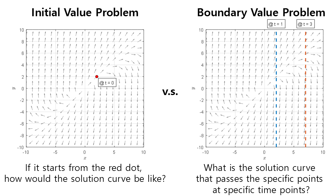
Figure 1. Comparison of initial value problems and boundary value problems

If we think about it, for an initial value problem, we just need to draw the solution curve along the given direction from the starting point. On the other hand, for a boundary value problem, we need to find the exact function that satisfies the given function values at the specified times. Therefore, a boundary value problem looks more difficult than an initial value problem.

We have found many solution curves for initial value problems, so let’s draw the solution curve for the boundary value problem given in equation (9), which can be obtained as shown in Figure 2 below (using the bvp4c solver in MATLAB).

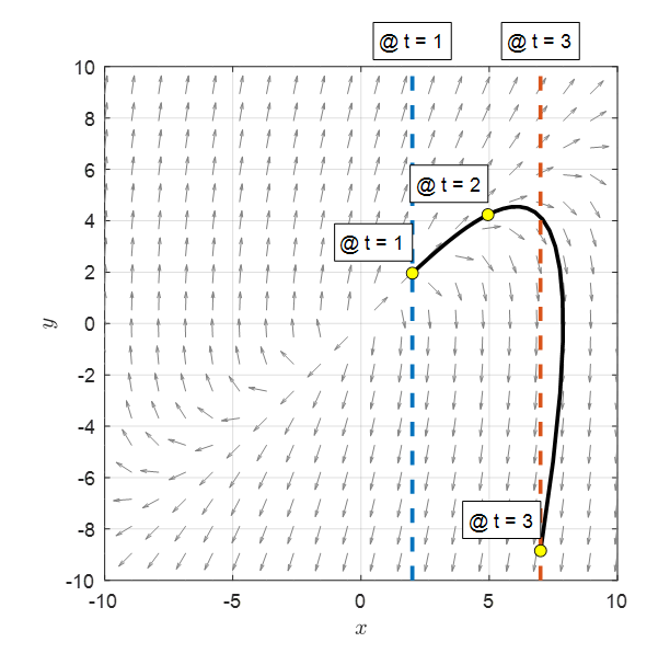
Figure 2. Solution curve for the given boundary value problem

Deriving the Analytic Solution of a Boundary Value Problem

From the perspective of obtaining the solution of a differential equation analytically, there seems to be little difference between a boundary value problem and an initial value problem.

For the following general solution,

\[\begin{bmatrix}x(t) \\ y(t) \end{bmatrix} = c_1 \begin{bmatrix}1 \\3 \end{bmatrix}e^{3t}+c_2\begin{bmatrix}1 \\ 1\end{bmatrix}e^t\]

if we substitute the boundary value conditions, we can obtain the following equation by applying the condition only to the first row of the above equation since the given condition is only for $x(t)$.

\[\text{at }t=1\text{, }x(1)=c_1e^3 + c_2 e=2\] \[\text{at }t=3\text{, }x(3)=c_1e^{3\cdot 3} + c_2 e^3=7\]

These two equations are equivalent to solving the following system of linear equations.

\[\begin{bmatrix}e^3 & e\\ e^9 & e^3\end{bmatrix}\begin{bmatrix}c_1 \\ c_2\end{bmatrix} = \begin{bmatrix}2 \\7\end{bmatrix}\]

Therefore, $c_1$ and $c_2$ are determined as follows.

\[\Rightarrow c_1 = -0.0010\text{, } c_2 = 0.7430\]

The equation for the solution curve obtained analytically is as follows, where $y(t)$ is determined by $y(t) = x’(t)$.

\[\begin{cases}x(t) = -0.001e^{3t}+0.7430e^{t} \\ y(t) = -0.003e^{3t}+0.7430e^{t}\end{cases}\]

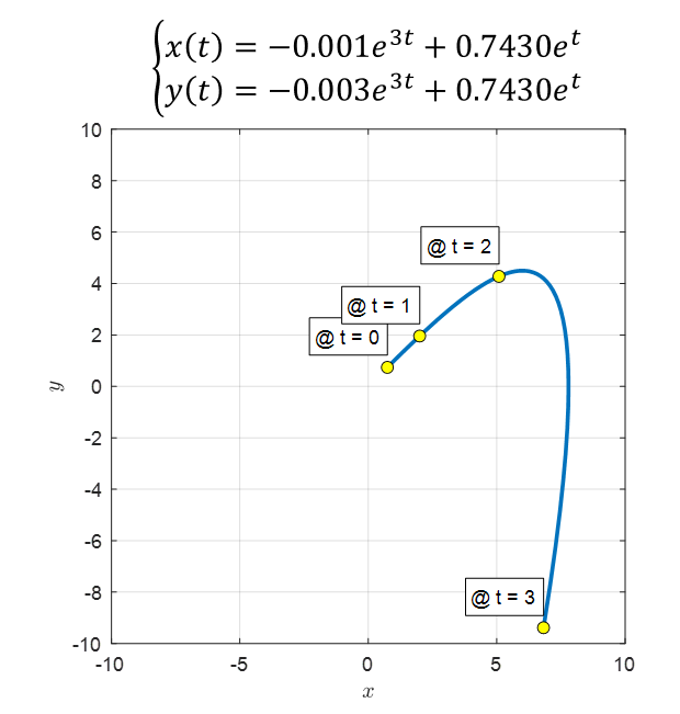
Figure 3. Solution curve for the given boundary value problem

We can see that this solution curve obtained analytically has a shape that is very similar to the curve obtained using the ODE solver shown in Figure 2.