※ In order to facilitate visualization and understanding, the field where vectors and matrices are defined is limited to real numbers.
Prerequisites
To fully understand this post, we recommend that you have knowledge of the following topics.
- Vector projection
Background Knowledge
Vector Projection
We learned about vector projection in high school mathematics.
In order for the concept of projection to be valid, we need two vectors.
The following figure shows the relationship between vector $a$ and vector $b$.
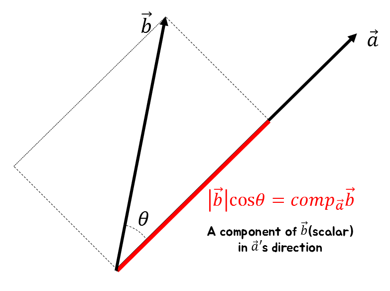
Figure 1. The component of one vector in the direction of another vector can be expressed using the cosine value.
For example, if we express vector $\vec{b}$ using vector $\vec{a}$ as shown in Figure 1, the component of $\vec{b}$ in the direction of $\vec{a}$ can be expressed as follows using the angle between the two vectors:
\[\text{comp}_{\vec{a}}\vec{b}=|\vec{b}|\cos\theta\]Meanwhile, the dot product of two vectors can be expressed as follows:
\[\vec{a}\cdot\vec{b} = |\vec{a}||\vec{b}|\cos\theta\]We can also see that the value of $|\vec{b}|\cos\theta$ can be expressed as follows:
\[|\vec{b}|\cos\theta = \frac{\vec{a}\cdot\vec{b}}{|\vec{a}|}=\text{comp}_{\vec{a}}\vec{b}\]On the other hand, $\text{comp}_{\vec{a}}\vec{b}$ is a scalar value. This can be seen from the fact that both $|\vec{b}|$ and $\cos\theta$ are scalar values.
If we want to obtain the vector value of the component of $\vec{b}$ in the direction of $\vec{a}$, what should we do?
We can simply multiply $\text{comp}_{\vec{a}}\vec{b}$ by the unit vector in the direction of $\vec{a}$.
If we denote the vector projection of $\vec{b}$ onto $\vec{a}$ as $\text{proj}_{\vec{a}}\vec{b}$, then its value is as follows. \(\text{proj}_{\vec{a}}\vec{b} = \text{comp}_{\vec{a}}\vec{b} \cdot \frac{\vec{a}}{|\vec{a}|} = |\vec{b}|\cos\theta\cdot \frac{\vec{a}}{|\vec{a}|}\)
On the other hand, it can be seen from equation (3) that:
\[\Rightarrow \text{proj}_{\vec{a}}\vec{b}=\frac{\vec{a}\cdot\vec{b}}{|\vec{a}|}\cdot \frac{\vec{a}}{|\vec{a}|}\] \[=\frac{\vec{a}\cdot\vec{b}}{|\vec{a}|^2}\vec{a}=\frac{\vec{a}\cdot\vec{b}}{\vec{a}\cdot\vec{a}}\vec{a}\]
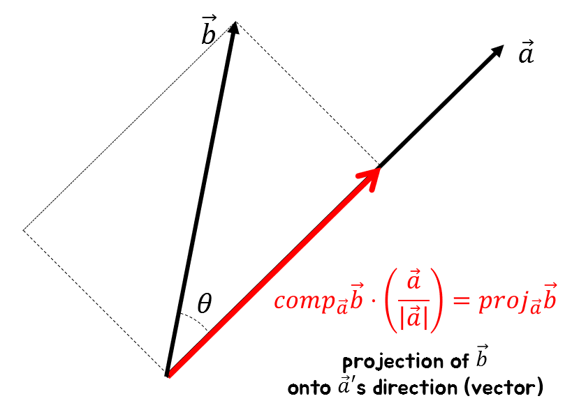
Figure 2. For one of two vectors, the component in the direction of another vector can be expressed using cosine values.
Gram-Schmidt Process
Consciousness of the Goal of the Gram-Schmidt Process
The Gram-Schmidt process essentially performs the following task when given linearly independent vectors:
“Let’s appropriately transform them to an orthogonal basis.”
This can be described using the following figure:
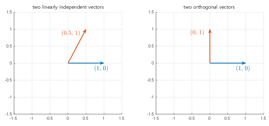
Figure 3. The Gram-Schmidt process is a process of transforming the two given vectors in the left figure to two orthogonal vectors as shown in the right figure.
Obtaining an orthogonal vector set has many advantages, but the most important is that compared to a non-orthogonal basis, obtaining an orthogonal basis has its own benefits.
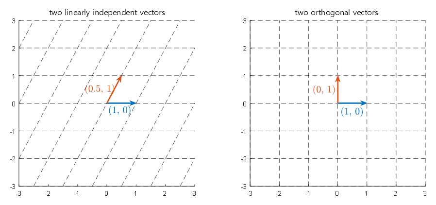
Figure 4. Left: Vector space generated using a non-orthogonal basis. Right: Vector space generated using an orthogonal basis.
Let’s say two linearly independent vectors $\lbrace v_1, v_2 \rbrace$ are a basis for a 2-dimensional real space. In this case, the two vectors do not need to be orthogonal to each other.
Then any vector $v\in \Bbb{R}^2$ in the 2-dimensional real space can be expressed as a linear combination of $v_1$ and $v_2$. In other words, $v$ can be represented using $v_1$ and $v_2$ as follows:
\[v = x_1v_1 + x_2 v_2 \text{ where } x_1, x_2 \in \Bbb{R}\]However, if we assume that two vectors $\lbrace w_1, w_2\rbrace$ form an orthonormal basis in a 2-dimensional real space, any arbitrary vector $v \in \Bbb{R}^2$ can be expressed as follows.
\[v = (v\cdot w_1)w_1 + (v\cdot w_2)w_2\]With this, we can easily obtain coefficients to represent $v$ as a linear combination of $v_1$ and $v_2$.
The process of Gram-Schmidt
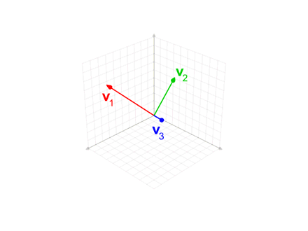
Figure 4. Animation representing the process of Gram-Schmidt orthonormalization
Source: Wikipedia, Gram-Schmidt process
The process of Gram-Schmidt can be expressed mathematically as follows.
Given linearly independent vectors $a_1, \cdots, a_k$ in a vector space $V$, we can construct a orthonormal basis as follows.
\[u_1 = a_1\] \[u_2 = a_2 - \text{proj}_{u_1}(a_2)\] \[u_3 = a_3 - \text{proj}_{u_1}(a_3) - \text{proj}_{u_2}(a_3)\] \[\vdots \notag\] \[u_k = a_k -\sum_{j=1}^{k-1}\text{proj}_{u_j}(a_k)\]The set of vectors generated in this way, $\lbrace u_1, u_2, \cdots, u_k \rbrace$, is orthogonal, and we can normalize each vector by dividing it by its norm.
That is,
\[q_i = \frac{u_i}{||u_i||}\]defines an orthonormal basis $\lbrace q_1, q_2, \cdots, q_k \rbrace$ for the vector space $V$.
Although it may look a bit complicated in mathematical notation, the essence of the equation is as follows.
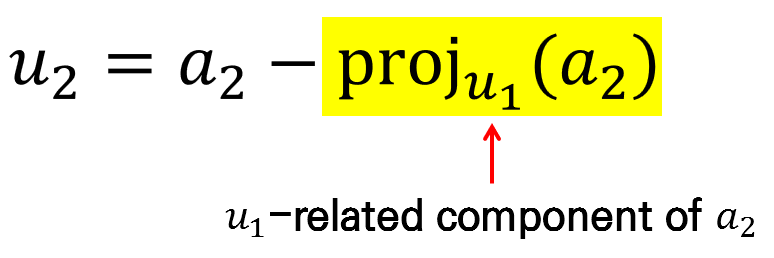
Figure 5. What the equation of Gram-Schmidt process tells you
To construct vectors that are orthogonal to each other, it is necessary to subtract each component that they occupy.
Once again, if you look at the picture, it is the same as Figure 6 below.
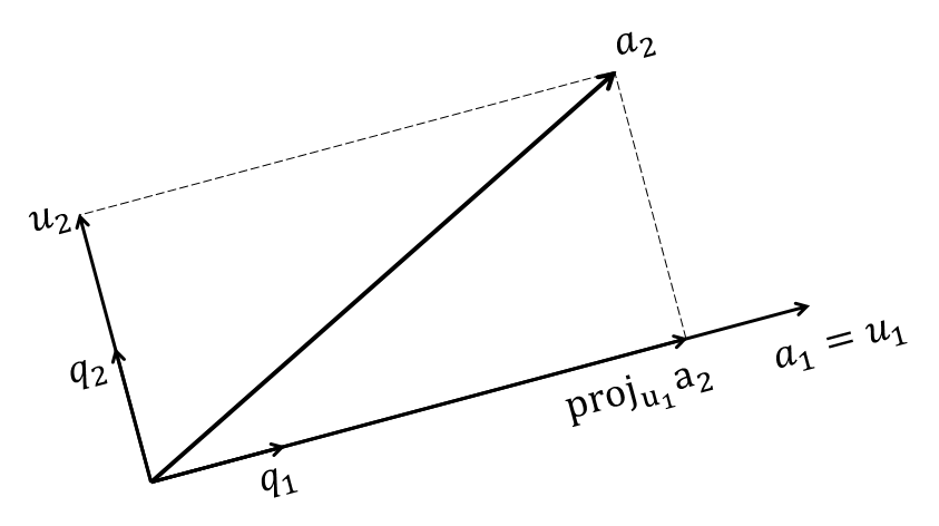
Figure 6. Basic principle of the Gram-Schmidt process
The Gram-Schmidt process allows us to iteratively find a new orthonormal basis vector for a given set of vectors.
QR decomposition
QR decomposition is a process of decomposing a matrix using orthonormal basis vectors found by the Gram-Schmidt process.
Let the orthonormal basis vectors obtained through the Gram-Schmidt process be denoted by $q_1, \cdots, q_n$, and let the matrix that collects them be denoted by $Q$. Then the following holds:
\[A = QR\] \[\begin{bmatrix} | & | & \text{ } & | \\ a_1 & a_2 &\cdots & a_n \\ | & | & \text{ } & | \end{bmatrix} = \begin{bmatrix} | & | & \text{ } & | \\ q_1 & q_2 &\cdots & q_n \\ | & | & \text{ } & | \end{bmatrix} \begin{bmatrix} a_1\cdot q_1 & a_2\cdot q_1 & \cdots & a_n\cdot q_1 \\ a_1\cdot q_2 & a_2\cdot q_2 & \cdots & a_n\cdot q_2 \\ \vdots & \vdots & \ddots & \vdots \\ a_1\cdot q_n & a_2\cdot q_n & \cdots & a_n\cdot q_n \\ \end{bmatrix}\]If we consider $a_1\cdot q_2$, the value is 0 since $q_2$ has removed all components of $a_1$ and $q_1$.
For the same reason, if $i<j$, then $a_i\cdot q_j=0$. This is because $q_j$ has removed all components of $a_i$ where $i<j$.
Therefore, the following equation holds:
\[=\begin{bmatrix} | & | & \text{ } & | \\ q_1 & q_2 &\cdots & q_n \\ | & | & \text{ } & | \end{bmatrix} \begin{bmatrix} a_1\cdot q_1 & a_2\cdot q_1 & \cdots & a_n\cdot q_1 \\ 0 & a_2\cdot q_2 & \cdots & a_n\cdot q_2 \\ \vdots & \vdots & \ddots & \vdots \\ 0 & 0 & \cdots & a_n\cdot q_n \\ \end{bmatrix}\]This is called QR decomposition.
Example Problem
It can be difficult to understand the explanation of QR decomposition in words alone, so let’s practice the Gram-Schmidt normalization process and QR decomposition through the example below.
Problem: Perform QR decomposition of the matrix $A$ below.
\[A = \begin{bmatrix}1 & 1 & 0\\ 1 & 0 & 1 \\ 0 & 1 & 1 \end{bmatrix}\]Let $a_1$, $a_2$, and $a_3$ be the column vectors of matrix $A$, as follows:
\[a_1 = \begin{bmatrix}1\\1\\0\end{bmatrix}, a_2 = \begin{bmatrix}1\\0\\1\end{bmatrix}, a_3 = \begin{bmatrix}0\\1\\1\end{bmatrix}\]For convenience, we will denote each column vector of $A$ as $a_1 = (1, 1, 0)$, etc.
To perform QR decomposition, let’s apply the Gram-Schmidt process to the three vectors.
Let’s denote the vectors obtained by orthogonalization but not normalization as $u_1$, $u_2$, etc., and the normalized orthonormal vectors as $e_1$, $e_2$, etc.
First, consider $a_1$:
\[a_1 = (1, 1, 0)\]According to the Gram-Schmidt process, we can use the first vector as it is.
\[u_1 = a_1=(1, 1, 0)\]Now let’s calculate $u_2$. $u_2$ is the vector obtained by subtracting the component of $a_2$ in the direction of $u_1$ from $a_2$.
\[u_2 = a_2 - \text{proj}_{u_1}a_2\] \[=(1, 0, 1) - \left(\frac{u_1\cdot a_2}{u_1\cdot u_1}\right)u_1\] \[=(1, 0, 1) - \frac{1\cdot1 + 1\cdot 0 + 0\cdot 1}{1^2+1^2+0^2}(1, 1, 0)\] \[=\left(\frac{1}{2}, -\frac{1}{2}, 1\right)\]Let’s also calculate $u_3$. $u_3$ is the vector obtained by subtracting the component of $a_3$ in the direction of $u_1$ and $u_2$ from $a_3$.
\[u_3 = a_3 - \text{proj}_{u_1}a_3 - \text{proj}_{u_2}a_3\] \[=(0, 1, 1) - \left(\frac{u_1\cdot a_3}{u_1\cdot u_1}\right)u_1-\left(\frac{u_1\cdot a_3}{u_2\cdot u_2}\right)u_2\] \[=(0, 1, 1) -\left(\frac{0+1+0}{1^2+1^2+0^2}\right)(1, 1, 0) - \left(\frac{(-1/2+1)}{1/4+1/4+1}\right)\left(\frac{1}{2}, -\frac{1}{2}, 1\right)\] \[(0, 1, 1) - \frac{1}{2}(1, 1, 0) -\frac{1}{3}\left(\frac{1}{2}, -\frac{1}{2}, 1\right)\] \[=\left(-\frac{2}{3},\frac{2}{3},\frac{2}{3}\right)\]To summarize, the vectors $u_1$, $u_2$, $u_3$ are as follows:
\[u_1 = (1, 1, 0), u_2 = \left(\frac{1}{2}, -\frac{1}{2}, 1\right), u_3 = \left(-\frac{2}{3},\frac{2}{3},\frac{2}{3}\right)\]Normalizing the above three vectors, we get:
\[e_1 = \frac{u_1}{\|u_1\|}=\frac{1}{\sqrt{2}}(1, 1, 0)=\left(\frac{1}{\sqrt{2}},\frac{1}{\sqrt{2}}, 0\right)\] \[e_2 = \frac{u_2}{\|u_2\|}=\sqrt{\frac{2}{3}}\left(\frac{1}{2},-\frac{1}{2}, 1\right)=\left(\frac{1}{\sqrt{6}},-\frac{1}{\sqrt{6}},\frac{2}{\sqrt{6}}\right)\] \[e_3 = \frac{u_3}{\|u_3\|}=\frac{1}{\sqrt{3\cdot(2/3)^2}}\left(-\frac{2}{3},\frac{2}{3},\frac{2}{3}\right)=\left(-\frac{1}{\sqrt{3}}, \frac{1}{\sqrt{3}},\frac{1}{\sqrt{3}}\right)\]Therefore, we can perform QR decomposition as follows, considering $e_1$, $e_2$, and $e_3$ as corresponding to $q_1$, $q_2$, and $q_3$ in $A=QR$.
\[A = QR =\begin{bmatrix} 1/\sqrt{2} & 1/\sqrt{6} & -1/\sqrt{3} \\ 1/\sqrt{2} & -1/\sqrt{6} & 1/\sqrt{3} \\ 0 & 2/\sqrt{6} & 1/\sqrt{3}\end{bmatrix}\begin{bmatrix}2/\sqrt{2} & 1/\sqrt{2} & 1/\sqrt{2} \\0 & 3/\sqrt{6} & 1/\sqrt{6} \\0 & 0 & 2/\sqrt{3}\end{bmatrix}\]Here, $Q$ is an orthonormal matrix and $R$ is an upper triangular matrix.