※ The concept called “divergence theorem” in this post refers to the 3-dimensional divergence theorem (Gauss’s theorem) unless otherwise specified. This is to distinguish it from the 2-dimensional divergence theorem.
Formula for Divergence Theorem
\[{\large\bigcirc}\kern-1.55em\iint_S\vec{F}\cdot d\vec{S} = \iiint_V(\vec{\nabla}\cdot\vec{F})dV\]Meaning of Divergence Theorem
Prerequisites
To understand the meaning of the divergence theorem, it is recommended to have knowledge of the following:
Introduction to the Meaning of Divergence Theorem
Suppose there is a closed surface S and a parallelepiped volume created by it on a vector field, as shown below on a 3-dimensional space.
Figure 1. Closed surface S and parallelepiped volume created by it on a vector field in a 3-dimensional space.
We can consider the surface vector for each of the six faces of the parallelepiped.
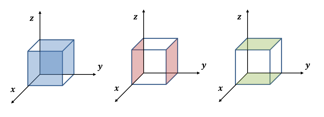
Figure 2. Six faces of the parallelepiped.
What we want to know in the divergence theorem is that the surface integral for these six faces is ultimately equal to the triple integral by the volume of the parallelepiped.
Like when we tried to understand the meaning of Green’s theorem or Stoke’s theorem by dividing the volume of the object, let’s think about the meaning of the divergence theorem by dividing the volume of the object into two along the y-axis as follows.
Figure 3. A volume divided into two parts along the y-axis.
Here, we can consider a total of 12 faces, but if we focus on the faces of the two divided parts, we can get an idea of what they look like as shown in Figure 4.
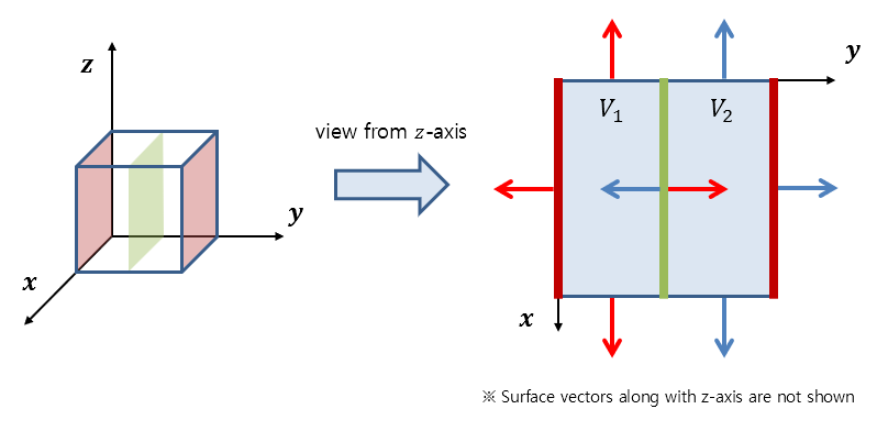
Figure 4. The shape of each face vector when the divided volume is viewed from the z-axis.
Let’s call the two divided volumes $V_1$ and $V_2$ and the six faces included in each volume $S_1$ and $S_2,” respectively.
As seen in Figure 4, the two face vectors coming out on each side of the divided faces have the same area but opposite directions, so the two surface integral values calculated on these faces add up to zero.
Therefore, if we add up all the surface integral values for the two volumes, we get the same value as the original (undivided) volume.
In other words, we can express this as follows:
\[{\large\bigcirc}\kern-1.55em\iint_S\vec{F}\cdot d\vec{S} ={\large\bigcirc}\kern-1.55em\iint_{S_1}\vec{F}\cdot d\vec{S_1} + {\large\bigcirc}\kern-1.55em\iint_{S_2}\vec{F}\cdot d\vec{S_2}\]Now, let’s divide the volume into four parts along the x and y axes, as shown in Figure 5.
Figure 5. A volume divided into four parts along the x and y axes.
Let’s call the divided volumes $V_1$ through $V_4$ and refer to the six faces included in each volume as $S_1$ through $S_4.”
As shown in Figure 6 below, we can see that for the internal faces of the divided volume, the two face vectors coming out on each side have the same area but opposite directions, so we can calculate the surface integral values for these faces and add them up to get zero.
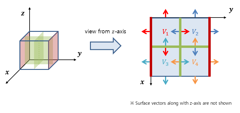
Figure 6. The shape of each face vector for the divided volume when viewed from the z-axis.
Therefore, if we add up the surface integral values of all four volumes, it will be equal to the surface integral value of the original (before splitting) volume.
In other words, it can be expressed as follows:
\[{\large\bigcirc}\kern-1.55em\iint_S\vec{F}\cdot d\vec{S} =\sum_{i=1}^{4}{\large\bigcirc}\kern-1.55em\iint_{S_i}\vec{F}\cdot d\vec{S_i}\]Continuing with the above discussion, we can split an arbitrary number of volumes in this way and the sum of the surface integral values of the split volumes will be equal to the surface integral value of the original volume. In other words, the following equation holds for any positive integer $N$:
\[{\large\bigcirc}\kern-1.55em\iint_S\vec{F}\cdot d\vec{S} =\sum_{i=1}^{N}{\large\bigcirc}\kern-1.55em\iint_{S_i}\vec{F}\cdot d\vec{S_i}\]
Figure 7. A rectangular solid split into an arbitrary number of volumes along the x and y axes
(in the figure, it is split into 1000 volumes)
Moreover, if we think inductively, the above discussion holds even when we split the volume into an infinite number of volumes. We can think of it as the sum of surface integral values of infinitely many split volumes being equal to the surface integral value of the original volume:
\[{\large\bigcirc}\kern-1.55em\iint_S\vec{F}\cdot d\vec{S} = \lim_{N\rightarrow \infty}\sum_{i=1}^{N}{\large\bigcirc}\kern-1.55em\iint_{S_i}\vec{F}\cdot d\vec{S_i}\]So, what does the value of the surface integral in a small volume mean?
The surface integral of a vector field calculates how similar the vector field vector passing through the differential surface area and the surface vector are by taking their dot product and adding it up over the entire curved surface.
Moreover, it was mentioned that the physical meaning of surface integral also represents the amount of fluid leaving through the curved surface S.
Furthermore, considering what we learned in divergence of a vector field, the meaning of divergence is the “amount of fluid leaving per unit volume.”
In other words, if this volume is very small, then the value of the divergence in the small volume multiplied by the volume of the small volume represents the amount of fluid leaving through the small volume.
Written in a formula, for an arbitrary very small volume $i$ with volume $\Delta V$, we have:
\[{\large\bigcirc}\kern-1.55em\iint_{S_i}\vec{F}\cdot d\vec{S_i} = (\vec{\nabla}\cdot\vec{F})\Delta V\]Now, if we consider the entire volume that is very small and divided into infinite pieces, equation (5) can be written as follows:
\[{\large\bigcirc}\kern-1.55em\iint_S\vec{F}\cdot d\vec{S} =\lim_{N\rightarrow \infty}\sum_{i=1}^{N}{\large\bigcirc}\kern-1.55em\iint_{S_i}\vec{F}\cdot d\vec{S_i}=\lim_{N\rightarrow \infty}\sum_{i=1}^{N}\left\lbrace(\vec{\nabla}\cdot\vec{F})\Delta V\right\rbrace\]In the end, adding $(\vec{\nabla}\cdot\vec{F})\Delta V$ for the given outermost volume means integrating over all $x$, $y$, and $z$ within this volume.
Also, as $N$ approaches infinity, $\Delta V$ can be written as $dV$. Therefore, we can derive the formula for the divergence theorem as follows:
\[{\large\bigcirc}\kern-1.55em\iint_S\vec{F}\cdot d\vec{S} = \iiint_V (\vec{\nabla}\cdot\vec{F})dV\]Proof of the Divergence Theorem
Prerequisites
To understand the proof of the Divergence Theorem, it is recommended to have knowledge of the following:
- Fundamental Theorem of Calculus
If $f$ is a continuous function on the closed interval $[a,b]$, and $F$ is any antiderivative of $f$, then the following holds:
\[\int_{a}^{b}f(t)dt = F(b) - F(a)\]- Divergence of a Vector Field
- Meaning of Multiple Integrals
- Normal Vector of a Differential Surface
- Surface Integral of a Vector Field
- Meaning of the Divergence Theorem
Introduction to the Surface, Domain, and Vector Field for the Proof
In this proof, we will use a closed cylindrical surface with a domain on the $x$-$y$ plane, and a height defined by $z = g_1(x,y)$ and $z=g_2(x,y)$ for the top and bottom surfaces of the cylinder, respectively. In particular, the normal vectors of the top and bottom surfaces of this closed surface (cylinder), determined by $g_1(x,y)$ and $g_2(x,y)$, respectively, are parallel to the unit vector of the $z$-axis 1.
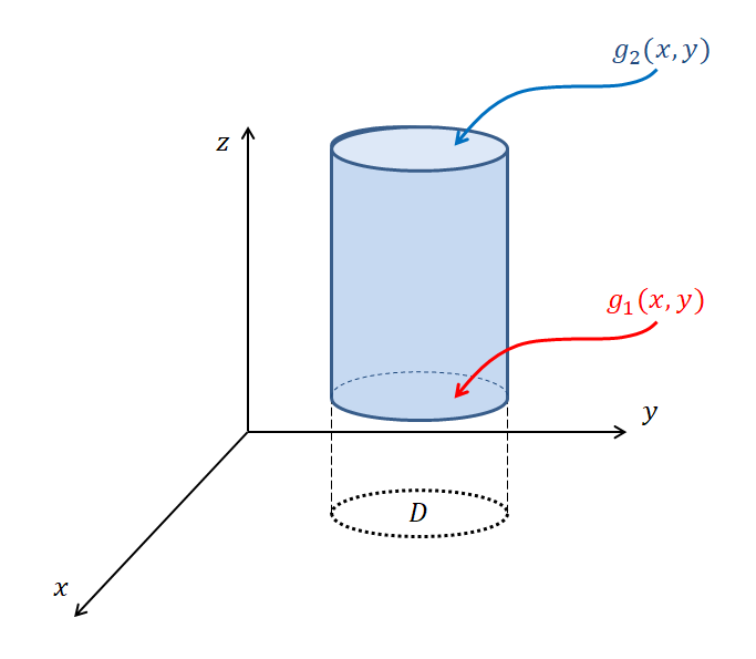
Figure 8. A closed cylindrical surface with a domain on the $x$-$y$ plane and a height defined by $z = g(x,y)$
Next, we can prove the Divergence Theorem for the general 3-dimensional space by applying a similar proof method as for the case where the domain is in the $x$-$y$ plane and the vector field is in the $\hat k$ direction, by also considering the cases where the domain is in the $y$-$z$ plane 2 and in the $x$-$z$ plane 3.
For this proof, let us assume that the vector field is given only in the $\hat k$ component. That is, we write the given vector field $\vec{F}$ on the 3-dimensional space as $\lt 0, 0, R\gt$. The angle brackets indicate that we have shortened the notation of the original $\vec{F} = R(x,y,z)\hat k$.
Let’s rewrite the Divergence Theorem formula we want to prove and start the proof.
\[{\large\bigcirc}\kern-1.55em\iint_S\vec{F}\cdot d\vec{S} = \iiint_V(\vec{\nabla}\cdot\vec{F})dV\]Proof using a given surface, domain, and vector field
Let’s start the proof of the divergence theorem from the surface integral part of the formula.
\[{\large\bigcirc}\kern-1.55em\iint_S\vec{F}\cdot d\vec{S}\]The closed surface we assume for the proof of the divergence theorem is cylindrical. Since the cylindrical surface can be divided into three parts - the top, side, and bottom surfaces - we can also write the above surface integral equation as follows:
\[{\large\bigcirc}\kern-1.55em\iint_S\vec{F}\cdot d\vec{S} = \iint_{S_\text{top}}\vec{F}\cdot d\vec{S} + \iint_{S_{side}}\vec{F}\cdot d\vec{S} + \iint_{S_{bottom}}\vec{F}\cdot d\vec{S}\]When considering the side surface integral, the normal vector of the surface is always parallel to the $x$-$y$ plane. However, the vector field we assume only has a $\hat k$ component, so the normal vector and the vector field are always perpendicular. Therefore, the side surface integral value is always 0. In other words, we can write it as follows:
\[{\large\bigcirc}\kern-1.55em\iint_S\vec{F}\cdot d\vec{S} = \iint_{S_\text{top}}\vec{F}\cdot d\vec{S} + \iint_{S_{bottom}}\vec{F}\cdot d\vec{S}\]Now, to expand the equation further, let’s calculate the surface vector ($d\vec{S}$) as we did in the surface integral of vector fields. Generally, the surface can be represented using two parameters as follows:
\[\vec{r}(u,v) = x(u,v)\hat i + y(u,v)\hat j + z(u,v)\hat k\]In this proof, the domain of the surface is $x$ and $y$, and the height is determined by $z = g_1(x,y)$ or $z=g_2(x,y)$. Therefore, we can express the equation of the surface as follows:
\[\vec{r}(x,y) = x\hat i + y\hat j + g(x, y)\hat k\]Therefore, the surface vector for an infinitesimal surface can be expressed as follows:
\[d\vec{S} = (r_x\times r_y) dxdy = \begin{vmatrix} \hat i && \hat j && \hat k \\ 1 && 0 && g_x \\ 0 && 1 && g_y\end{vmatrix} dxdy\] \[=\lt -g_x, -g_y, 1 \gt dxdy\]Let’s now expand the calculation of the original surface integral equation.
\[\Rightarrow \iint_{S_\text{top}}\vec{F}\cdot d\vec{S} + \iint_{S_{bottom}}\vec{F}\cdot d\vec{S} \notag\] \[=\iint_{D_{top}}\lt 0, 0, R(x, y, g_2(x,y))\gt \cdot \lt -g_x, -g_y, 1\gt dxdy\notag\] \[-\iint_{D_{bottom}}\lt 0, 0, R(x, y, g_1(x,y))\gt \cdot \lt -g_x, -g_y, 1\gt dxdy\]The sign change in the middle of the equation from addition to subtraction is due to the fact that the normal vector of $g_2(x,y)$ and the normal vector of $g_1(x, y)$ are in opposite directions.
After taking the dot product, the equation can be further developed as follows:
\[\Rightarrow\iint_{D_{top}}R(x,y,g_2(x,y))dxdy - \iint_{D_{bottom}}R(x,y,g_1(x,y))dxdy\] \[=\iint_D R(x,y,g_2(x,y)) - R(x,y,g_1(x,y))dxdy\]Similar to the approach used in the proof of the Green’s Theorem, this equation can also be thought of by using the fundamental theorem of calculus in calculus.
\[\Rightarrow\iint_D \left(\int_{z=g_1(x,y)}^{z=g_2(x,y)} \frac{\partial R}{\partial z}dz\right) dxdy\]This can be expressed as follows using triple integration.
\[\Rightarrow \iiint_V\frac{\partial R}{\partial z}dxdydz\]Here, $\frac{\partial R}{\partial z}$ is equal to the divergence value of the vector field $\vec{F} = \lt 0, 0, R\gt$. Also, $dxdydz$ is a small volume, so it can be written as $dV$. Therefore, the above equation can be written as follows.
\[\Rightarrow \iiint_V\left(\vec{\nabla}\cdot \vec{F}\right)dV\]In other words, this is equivalent to proving the original divergence theorem equation.
Divergence Theorem for General 3D Spaces
We have proven the divergence theorem for a vector field with a domain in $x$, $y$ and a component in the direction of the $z$ axis 1. Similarly, for a vector field with a domain in $y$, $z$ and a component in the direction of the $x$ axis 2, and for a vector field with a domain in $x$, $z$ and a component in the direction of the $y$ axis 3, the divergence theorem for closed surfaces in 3D space can be proven using the same method.