This post is a summary of Professor S. C. Duta Roy’s lecture at IIT, which can be found at https://www.youtube.com/watch?v=vpPbaw9k8PY&ab_channel=nptelhrd.

1. Analog Filter

a. General Analog Systems and Filters

Before discussing analog filters, it is important to understand how general analog systems are modeled. This is because the shape of an analog system ultimately determines the shape of the analog filter. It is also important to establish what is meant by “general analog signals or systems” in this post. In this post, a general analog system refers to a linear time-invariant system. This means it represents a signal that is substantially exactly determined without external noise. Typically, a general LTI model represented as

\[x(t) \rightarrow h(t)\rightarrow y(t)\]

can also be expressed as follows:

\[y(k) = -\sum_{n=1}^{N}a_ny(k-n)+\sum_{n=0}^Nb_nx(k-n)\]

At this point, the system can also be expressed through its impulse response, as shown below:

\[Y(j\Omega) = H(j\Omega)X(j\Omega)\]

Both $Y(j\Omega)$ and $X(j\Omega)$ can also be expressed as:

\[Y(j\Omega) = Y(s) = a_ns^n + a_{n-1}s^{n-1}+\cdots+a_1s^1 + a_0\] \[X(j\Omega) = X(s) = b_ns^n + b_{n-1}s^{n-1}+\cdots+b_1s^1 + a_0\]

Therefore, a general system $H(j\Omega)$ can also be expressed as:

\[H(s) \frac{\sum_{i=0}^{q}b_is^{-i}}{\sum_{k=0}^{p}a_ks^{-k}}\]

On the other hand, filters can also be thought of as a type of system. This is because a system that is specially manipulated can perform the function of a filter, with respect to the role of the system and the role of the filter. If we think about the role or function of the filter, it can be said that it performs the function of amplifying or maintaining desired information while attenuating or removing undesired information. An appropriately manipulated system can be used as a filter. Therefore, an analog filter can be defined as follows:

\[H_a(s) = G\frac{1+d_1s^{-1}+\cdots d_qs^{-q}}{1+c_1s^{-1}+\cdots+c_qs^{-q}}\]

Analog filters of this type are usually called IIR filters.

To reiterate, if the coefficients of $H_a(s)$ are properly adjusted, it can function as a filter. Many types of filters have been invented through extensive research, and among them, the most commonly used IIR filters are the Butterworth filter and the Chebyshev filter.

The general formula for the Butterworth filter is as follows:

\[|H_a(j\Omega)|^2 = 1 / \left\lbrace 1+\left(\frac{\Omega}{\Omega_c}\right)^{2N}\right\rbrace\]

The general formula for the Chebyshev filter is as follows:

\[|H_a(j\Omega)|^2 = 1/ \left\lbrace1+\epsilon^2C^2_N\left(\frac{\Omega}{\Omega_p}\right)\right\rbrace\]

First, let’s take a look at the Butterworth filter, which simplifies life.

2. All-pole filters

Take a good look at the formula for the Butterworth filter. We can see that it is quite different from the general shape of a filter model. It can start with the fact that all elements in the numerator part of the general filter formula are gone, leaving only 1.

And all elements that make up the filter are only in the denominator. The s elements in the numerator are generally called zeros, and the s elements in the denominator are called poles. Since the Butterworth filter only has poles and the zeros are nowhere to be found, this type of filter is called an all-pole filter. So why was the all-pole filter invented, and why did it end up being the final product over all-zero filters?

The answer to this question is that all types of filters (low-pass filters, high-pass filters, band-pass filters, notch filters) can all be derived from the low-pass filter, so if we can mathematically construct a basic low-pass filter (which we will study later on with the normalized low-pass filter), we can construct the rest of the filters. So what is the relationship between the low-pass filter and the all-pole filter? It is because the pole specifies the passband.

In other words, the input function survives as an output function when it passes through the point where the pole is generated. In contrast, the input function disappears as it passes through the point where the zero is generated. So why do we discuss zeros in all-pole filters where there are no zeros? That is because filters that only have poles or only have zeros do not exist.

3. Filter specification

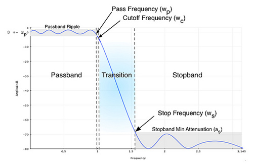
Source: SPrelated.com / Python scipy.signal IIR filter Design

So far, we’ve learned that a filter is a kind of system, and we’ve learned that there are two most commonly used types of filters. We have also learned that by adjusting the coefficients of this system appropriately, we can make it a filter and use it. Then, how should we adjust these coefficients appropriately? We cannot help but think about what we are going to adjust these coefficients for.

Generally, a filter must be born with the mission of preserving the desired frequency range and killing the frequency range that should not come out. This can be demanded through filter specification. The perfect filter is a filter that has a slope perpendicular to the transition and only passes through the frequency components of the part to be passed. However, such a filter does not exist. There are several reasons why this is so.

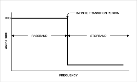
The ideal filter looks like the above. It looks simple in the frequency domain without any major problems, but when it is reverse Fourier transformed back into the time domain, we find that such a filter cannot actually exist. This is because the filter that is reverse Fourier transformed from the ideal filter is a sinc function. The general sinc function is not causal and has an infinite impulse response.

Anyway, to create a practical filter system, it is more important to create a compromise filter that is appropriately constructed. So, we ask the engineer to construct a filter with a passband frequency at -2dB and a stopband frequency at -40dB using the decibel. With this requirement, let’s study how to adjust the order of the Butterworth filter and how to adjust the cutoff frequency ($\Omega_c$).

4. The shape of the Butterworth filter and how to satisfy specifications

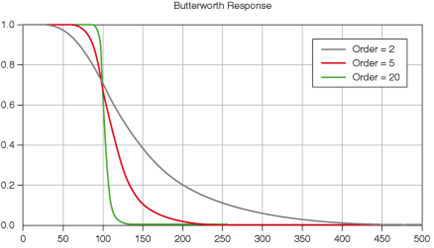
Generally, the shape of the Butterworth filter is as shown above. We can just say, “Wow, this is what it looks like!” and use it, but before that, we need to mathematically confirm how we can create such a shape. Let’s think about the equation of the Butterworth filter again.

\[|H_a(j\Omega)|^2 = 1 / \left\lbrace 1+\left(\frac{\Omega}{\Omega_c}\right)^{2N}\right\rbrace\]

One thing we can do first is to differentiate the Butterworth filter equation at $\Omega=0$ and $\Omega=\infty$ to see how the slope behaves at both ends.

First, let’s simplify the equation a bit.

\[|H_a(j\Omega)|=\left[1+\left(\frac{\Omega}{\Omega_c}\right)^{2N}\right]^{1/2}\]

Then, let’s differentiate both sides with respect to $\Omega$.

\[\frac{d}{d\Omega}|H_a(j\Omega)| = \left[-\frac{1}{2}+\left(\frac{\Omega}{\Omega_c}\right)^{-3/2}\right]\left[2N\left(\frac{\Omega}{\Omega_c}\right)^{2N-1}\right]\left(\frac{1}{\Omega_c}\right)\] \[\therefore \left|\frac{d}{d\Omega}|H_a(j\Omega)|\right|_{\Omega = 0} = 0\]

Therefore, we can see that the Butterworth filter is flat at $\Omega=0$, and this is valid for all higher-order derivatives, making it maximally flat.

On the other hand, what happens when $\Omega\rightarrow\infty$?

\[|H_a(j\Omega)| = 1/\sqrt{1+\left(\frac{\Omega}{\Omega_c}\right)^{2N}}\]

Therefore,

$\lim_{\Omega\rightarrow \infty}|H_a(j\Omega)|$ follows the magnitude of $\left(\frac{\Omega}{\Omega_c}\right)^{-N}$, so it converges to 0. Looking at it in decibels, we have:

\[\lim_{\Omega\rightarrow \infty}|H_a(j\Omega)| = -20N \log_{10}\left(\frac{\Omega}{\Omega_c}\right)\]

Thus, we can think of it as an asymptotic line that gradually decreases in proportion to the value of -20N. In addition, as N increases, the denominator grows rapidly, making the transition steeper and closer to the ideal filter shape.

Therefore, we can imagine a plot of a Butterworth filter similar to the one in the above figure. This way, we have mathematically thought about the shape of the Butterworth filter. However, understanding this does not necessarily mean that we can match the filter specifications. Let’s think more about the filter specification.

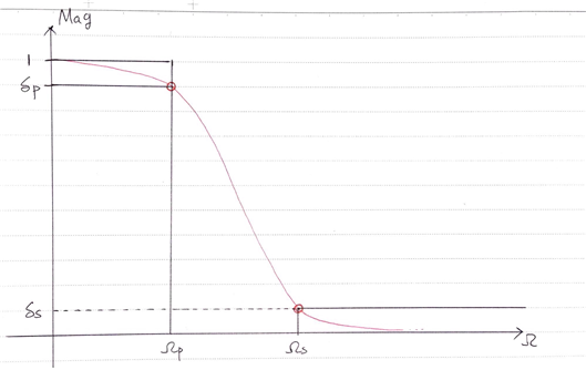
For a general Butterworth filter, it is known that regardless of the order of the Butterworth filter, it passes through $(\Omega_p,\delta_p)$ and $(\Omega_s,\delta_s)$. Therefore, we can derive two equations. From the general equation (10) of the Butterworth filter,

① When $\Omega=\Omega_p$,

\[1/\left\lbrace1+\left(\frac{\Omega_p}{\Omega_c}\right)^{2N}\right\rbrace=\delta^2_p\]

② When $\Omega=\Omega_s$,

\[1/\left\lbrace1+\left(\frac{\Omega_s}{\Omega_c}\right)^{2N}\right\rbrace=\delta^2_s\]

Taking the reciprocal of both equations and rearranging the terms, we can obtain:

From Equation (16),

\[\left(\frac{\Omega_p}{\Omega_c}\right)^{2N} = \delta_p^{-2}-1\]

From Equation (17),

\[\left(\frac{\Omega_s}{\Omega_c}\right)^{2N} = \delta_s^{-2}-1\]

We can then express Equations (18) and (19) as the ratio of the two equations:

\[\left(\frac{\Omega_p}{\Omega_s}\right)^{2N} = \frac{\delta^{-2}_p-1}{\delta_s^{-2}-1}\]

By taking the logarithm of both sides of Equation (20) with a base of 10, we can derive the value of $N$.

\[2N = \log_{10}\left(\frac{\delta^{-2}_p-1}{\delta_s^{-2}-1}\right) / \log_{10}\left(\frac{\Omega_p}{\Omega_s}\right)\] \[N = \frac{1}{2}\log_{10}\left(\frac{\delta^{-2}_p-1}{\delta_s^{-2}-1}\right) / \log_{10}\left(\frac{\Omega_p}{\Omega_s}\right)\] \[N = \log_{10}\sqrt{\frac{\delta^{-2}_p-1}{\delta_s^{-2}-1}} / \log_{10}\left(\frac{\Omega_p}{\Omega_s}\right)\]

However, since N is an integer, the formula that satisfies the practical N that can be used is

\[N \geq\log_{10}\sqrt{\frac{\delta_p^{-2}-1}{\delta_s^{-2}-1}} / \log_{10}\left(\frac{\Omega_p}{\Omega_s}\right)\]

and the minimum N that satisfies the above formula should be found.

Also, if we know the cutoff frequency $\Omega_c$, we can design a Butterworth filter that meets the desired specifications.

To obtain $\Omega_c$, the filter function must always pass through $(\Omega_p, \delta_p)$.

One might think that it does not pass through $(\Omega_s, \delta_s)$. However, in reality, since the condition of N is an integer that satisfies formula (24), the filter is designed so that it cannot pass through $(\Omega_s, \delta_s)$.

Therefore, when obtaining $\Omega_c$, it is practical and desirable to search for the condition that passes through $(\Omega_p, \delta_p)$. Thus, $\Omega_c$ can be found by satisfying the equation

\[1/\left\lbrace 1+\left(\frac{\Omega_p}{\Omega_c}\right)^{2N}\right\rbrace = \delta_p^2\]

from the formula

\[\left(\frac{\Omega_p}{\Omega_c}\right)^{2N} = \delta_p^{-2}-1.\]

We have briefly looked at the shapes of the Butterworth filter at $\Omega=0$ and $\Omega=\infty$ and how to find N and $\Omega_c$ that meet the specifications.

Can we design an analog filter system now that we know N and $\Omega_c$? The answer is ‘not yet possible’.

This is because when designing analog systems, we generally need to know the system’s equation in terms of Laplace frequency, s.

The equation of a system defined using Laplace frequency is generally referred to as the Transfer function.

5. Butterworth filter’s transfer function (s-domain)

First, we can map the Butterworth filter to the s-domain from formula (10) and derive the general analog filter $|H_a(s)|$ by only taking stable values of s. Then, let’s look at the process of deriving the general formula for $|H_a(s)|$.

First, we can easily represent the Butterworth filter in the s-domain through the transformation of $s=j\Omega$. That is, the following equation holds.

\(|H_a(j\Omega)|^2 = H_a(s)H_a(-s)\) Here’s a translation of the passage:

The reason for dividing the expression into the parts with “s” and “-s” will become clear later, but s can be split into a complex conjugate pair of $\pm$, and only the positive values of s are stable. Therefore, we can generalize the expression as:

\[H_a(s) H_a(-s) = 1/\left\lbrace 1+\left(\frac{-s^2}{\Omega_c^2}\right)^N\right\rbrace\]

If we can determine the values of the poles expressed as “s” and represent the generalized $|H_a(s)|$ in terms of these poles, we can obtain the transfer function of the Butterworth filter in the s-domain for any N.

Poles are defined as the values of s that make the denominator of the expression equal to zero. Thus, the poles of the Butterworth filter can be defined as s that satisfy the following expression:

\[1+\left(\frac{-s^2}{\Omega_c^2}\right)^N = 0\] \[\Rightarrow \left(\frac{-s^2}{\Omega_c^2}\right)^N = (-1) = \exp\left(j(2k-1)\pi\right)\text{ for } k = 1, 2, \cdots, N\] \[\Rightarrow \left(\frac{-s^2}{\Omega_c^2}\right)=\exp\left(j\frac{2k-1}{N}\pi\right)\] \[s_k^2 = -\Omega_c^2\exp\left(j\frac{2k-1}{N}\pi\right)\text{ for }k= 1, 2, \cdots, N\] \[\therefore s_k = \pm j\Omega_c^2\exp\left(j\frac{2k-1}{2N}\pi\right)\text{ for }k= 1, 2, \cdots, N\]

In this context, $s_k$ can be divided into two types: positive values and negative values. However, when $s_k$ has positive values, all of them exist in the Left Hand Plane of the s-plane, which means that only positive $s_k$ can constitute a stable system. ¹

Therefore, I will prove that positive $s_k$ always exists in the Left Hand Plane. Since positive $s_k$ always exists in the Left Hand Plane, it can be inferred that negative $s_k$ always exists in the Right Hand Plane, so I will omit the proof.

---

PROOF 1: The location of positive $s_k$ in the $s$-domain

For positive $s_k$,

\[s_k^+= j\Omega_c\exp\left(j\frac{2k-1}{2N}\pi\right)\text{ for }k = 1, 2, \cdots, N\] \[=j\Omega_c\left(\cos\left(\frac{2k-1}{2N}\pi\right)+j\sin\left(\frac{2k-1}{2N}\pi\right)\right)\] \[=\Omega_c\left(j\cos\left(\frac{2k-1}{2N}\pi\right)-\sin\left(\frac{2k-1}{2N}\pi\right)\right)\]

Here, you can easily find that the following is true.

\[\sin\left(\frac{2k-1}{2N}\pi\right) = \left\lbrace \sin\left(\frac{1}{2N}\pi\right), \text{ } \sin\left(\frac{3}{2N}\pi\right), \text{ } \sin\left(\frac{5}{2N}\pi\right), \cdots, \text{ } \sin\left(\frac{2N-1}{2N}\pi\right) \right\rbrace\]

However, all $\sin\left(\frac{2k-1}{2N}\pi\right)$ values are located in the first and second quadrants, and these values are all positive. Therefore, the real part of $s_k$ always takes on negative values.

Thus, $s_k^+=j\Omega_c\exp\left(j\frac{2k-1}{2N}\pi\right)$ is always a Left Hand Pole in the $s$-plane, regardless of the value of $N$.

Q.E.D.

---

Therefore, generally, by using the pole values of

\[s_k = \Omega_c\left(-\sin\left(\frac{2k-1}{2N}\pi\right)+j\cos\left(\frac{2k-1}{2N}\pi\right)\right)\text{ for }k = 1, 2, \cdots, N\]

a stable Butterworth system can be constructed.

Therefore, a generally stable Butterworth filter system can be defined in the $s$-domain as follows.

\[H_a(s) = 1/\left\lbrace1+\left(\frac{s}{\Omega_c}\right)^N\right\rbrace\] \[=\Omega_c / \left\lbrace\prod_{k=1}^{N}\left(\frac{s}{\Omega_c} - \hat{s}_k\right)\right\rbrace\notag\] \[\text{ where } \hat{s}_k = \Omega_c\left(-\sin\left(\frac{2k-1}{2N}\pi\right) + j\cos\left(\frac{2k-1}{2N}\right)\pi\right)\]

Or you can define it as below.

\[H_a(s) = 1/\prod_{k=1}^{N}\left(\frac{s}{\Omega_c}-s_k\right)\notag\]

\(\text{ where } s_k = -\sin\left(\frac{2k-1}{2N}\pi\right) + j\cos\left(\frac{2k-1}{2N}\pi\right)\) Therefore, if we consider each value of $N$ separately, we can express it as follows:

For $N=1$,

\[H_a(s) = 1/\left(\frac{s}{\Omega_c}-s_1\right)\notag\] \[\text{ where }s_1 = -\sin\left(\frac{1}{2}\pi\right)+j\cos\left(\frac{1}{2}\pi\right)=-1+0j = -1\] \[\therefore H_a(s) = 1/\left(\frac{s}{\Omega_c}+1\right)=\frac{\Omega_c}{s+\Omega_c}\]

For $N=2$,

\[H_a(s) = 1/\left\lbrace\prod_{k=1}^{2}\left(\frac{s}{\Omega_c}-s_k\right)\right\rbrace = 1/\left\lbrace\left(\frac{s}{\Omega_c}-s_1\right)\left(\frac{s}{\Omega_c}-s_2\right)\right\rbrace\]

where

\[s_1 = -\sin\left(\frac{1}{4}\pi\right)+j\cos\left(\frac{1}{4}\pi\right)\] \[=-\frac{\sqrt{2}}{2}+j\frac{\sqrt{2}}{2}\] \[s_2 = -\sin\left(\frac{3}{4}\pi\right)+j\cos\left(\frac{3}{4}\pi\right)\] \[=-\frac{\sqrt{2}}{2}-j\frac{\sqrt{2}}{2}\]

Therefore,

\[\therefore H_a(s) = \left\lbrace1/\left(\frac{s}{\Omega_c}+\frac{\sqrt{2}}{2}-j\frac{\sqrt{2}}{2}\right)\right\rbrace \left\lbrace1/\left(\frac{s}{\Omega_c}+\frac{\sqrt{2}}{2}+j\frac{\sqrt{2}}{2}\right)\right\rbrace\] \[=\Omega_c^2 / \left(s^2 + \sqrt{2}s\Omega_c + \Omega_c^2\right)\]

In the case of $N=3$, when we get to this point, we are quite tired. Let’s try a little trick. First, let’s set $\Omega_c=1$, and then substitute $s = \frac{s}{\Omega_c}$, which gives the same result. This method is called the denormalization method, which will be learned later.

\[H_a(s)|_{\Omega_c = 1} = 1/\prod_{k=1}^{N}(s-s_k)\] \[=\frac{1}{(s-s_1)(s-s_2)(s-s_3)}\]

where

\[s_1 = -\sin\left(\frac{1}{6}\pi\right)+j\cos\left(\frac{1}{6}\pi\right) = -\frac{1}{2}+j\frac{\sqrt{3}}{2}\] \[s_2 = -\sin\left(\frac{3}{6}\pi\right) + j \cos\left(\frac{3}{6}\pi\right) = -1\] \[s_3 = -\sin\left(\frac{5}{6}\pi\right)+j\cos\left(\frac{5}{6}\pi\right)=-\frac{1}{2}-j\frac{\sqrt{3}}{2}\]

Therefore, if we substitute $s_1$, $s_2$, and $s_3$ into the equation, we get

\[H_a(s) = 1/\left[(s+1)\left\lbrace(s+\frac{1}{2})^2 + \frac{3}{4}\right\rbrace\right]\] \[=\frac{1}{(s+1)(s^2 + s + 1)}\] \[=\frac{1}{s^3 + 2s^2 + 2s + 1}\]

If we substitute $s = s/\Omega_c$, we can see that

\[H_a(s) = \frac{\Omega_c^3}{s^3 + 2\Omega_cs^2 + 2\Omega_c^2s + \Omega_c^3}\]

Up to this point, we can see that there is a difference in the pole values between cases where $N$ is odd and even. If $N$ is odd, there is one pole that is a real number, and the rest are all complex numbers. If $N$ is even, all poles are complex numbers. The reason for this is as follows.

From the follwoing equation,

\[s_k = -\sin\left(\frac{2k-1}{2N}\pi\right)+j\cos\left(\frac{2k-1}{2N}\pi\right)\]

There must be points that satisfy following condition.

\[\frac{2k-1}{2N}\pi = \frac{1}{2}\pi\]

Thus, when $N$ is odd, $s_k$ must be $-1$ at $k=(N+1)/2$. Moreover, in general,

\[\cos\left(\pi-\theta\right)=-\cos(\theta)\] \[\sin\left(\pi-\theta\right)=\sin(\theta)\]

which means that all $s_p$ are complex conjugates of $s_{N-p+1}$.

Therefore, we can say that $S_{N-p+1} = s^*_p$. Additionally,

\[s_p+s^*_p = 2\sin\left(\frac{2k-1}{2N}\pi\right)\]

and

\[s_ps^*_p=1\]

are true properties.

Hence, we can consider $H_a(s)$ as follows.

When N is even,

\[H_a(s) = \Omega_c^N / \left\lbrace\prod_{k=1}^{N/2}\left(s^2 + b_k\Omega_c s + \Omega_c^2\right)\right\rbrace\notag\] \[\text{ where }b_k = 2\sin\left(\frac{2k-1}{2N}\pi\right)\]

When N is odd,

\[H_a(s) = \Omega_c^N / \left\lbrace(s+\Omega_c) \prod_{k=1}^{\frac{N-1}{2}}\left(s^2 + b_k\Omega_c s + \Omega_c^2\right)\right\rbrace\notag\] \[\text{ where }b_k = 2\sin\left(\frac{2k-1}{2N}\pi\right)\]

Thus, we have derived the general transfer function of the Butterworth Filter in the s-domain.

---

In summary,

\[N \geq\log_{10}\sqrt{\frac{\delta^{-2}_p-1}{\delta_s^{-2}-1}} / \log_{10}\left(\frac{\Omega_p}{\Omega_s}\right)\]

can be used to determine N, and

\[\left(\frac{\Omega_p}{\Omega_c}\right)^{2N} = \delta_p^{-2}-1\]

can be used to determine $\Omega_c$.

Furthermore, by using the expressions above, we can define the Butterworth filter in the general $s$-domain, where $N$ is even,

\[H_a(s) = \Omega_c^N / \left\lbrace\prod_{k=1}^{N/2}\left(s^2 + b_k\Omega_c s + \Omega_c^2\right)\right\rbrace\notag\] \[\text{ where }b_k = 2\sin\left(\frac{2k-1}{2N}\pi\right)\]

and $N$ is odd,

\[H_a(s) = \Omega_c^N / \left\lbrace(s+\Omega_c) \prod_{k=1}^{\frac{N-1}{2}}\left(s^2 + b_k\Omega_c s + \Omega_c^2\right)\right\rbrace\notag\] \[\text{ where }b_k = 2\sin\left(\frac{2k-1}{2N}\pi\right)\]

This enables us to define the Butterworth filter in the general $s$-domain.