Markov’s Inequality

Markov’s inequality is an inequality that holds for non-negative random variables. The definition of Markov’s inequality is as follows:

Let $X$ be a non-negative random variable and let $\alpha\gt 0$¹ be any constant that satisfies the condition. Then, the following inequality holds:

\[P(X\geq \alpha) \leq E[X]/\alpha\]

To understand the meaning of the above equation, let’s look at the figure below.

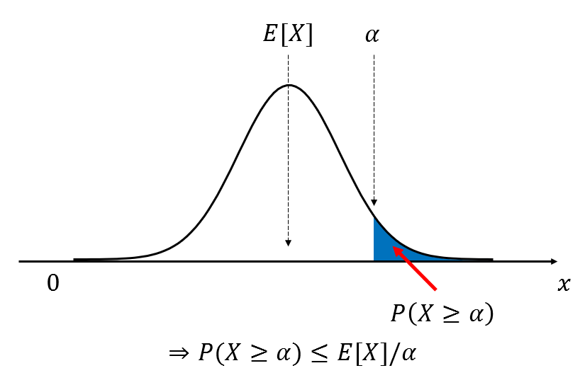
Figure 1. Markov's inequality represents the probability that a random variable $x$ is greater than some extreme value $\alpha$ with respect to the expected value in the entire data distribution.

From Figure 1, we can see that the pdf of a random variable $X$ is drawn. Here, we emphasized that $X$ is a non-negative value by indicating 0 on the left axis. In addition, the expected value was arbitrarily set to the middle of the distribution, and $P(X\geq \alpha)$ is shown in blue.

In summary, Markov’s inequality can be regarded as a theorem that describes the probability that a non-negative random variable $X$ is greater than some extreme value $\alpha$ with respect to the expected value.

The proof is very simple. If the pdf of $X$ is denoted by $f_X(x)$, then its expected value is as follows:

\[E[X]=\int_x x f_X(x)dx\]

The integral range can be divided into two parts with $\alpha$ as the boundary as follows:

\[\Rightarrow \int_{0\leq x \lt \alpha}xf_X(x)dx + \int_{X\geq \alpha}xf_X(x)dx\]

Here, the value of $x$ is always a non-negative value, so the left term of the above equation is always positive. Therefore, the following relation holds:

\[\Rightarrow \int_{0\leq x \lt \alpha}xf_X(x)dx + \int_{X\geq \alpha}xf_X(x)dx \geq \int_{X\geq \alpha}xf_X(x)dx\]

Furthermore, since $X\geq \alpha$ in the right-hand side of the above equation, the following holds:

\[\Rightarrow \int_{X\geq \alpha}xf_X(x)dx\geq \int_{X\geq \alpha}\alpha f_X(x)dx % Equation (5)\]

Therefore, if we only take Equation (2) and Equation (5), we have:

\[\Rightarrow E[X]\geq \int_{x\geq \alpha} \alpha f_X(x)dx % Equation (6)\]

According to the definition of pdf and probability, the above equation can also be written as follows.

\[\text{Equation} (6)\Rightarrow E[x]\geq \alpha P(X\geq \alpha) % 식 (7)\]

Here, tidying up the equation above leads to equation (1).

Chebyshev Inequality

Derivation of Chebyshev Inequality

The Chebyshev inequality states that for any random variable $X$ and any constant $\alpha$, the following inequality holds:

\[P(\left|X-E[X]\right|\geq\alpha)\leq Var[X]/\alpha^2 % Equation (8)\]

Unlike the Markov inequality, the Chebyshev inequality is a two-sided inequality in terms of the extreme values $E[X]\pm\alpha$ of $X$, as can be seen from the absolute value signs.

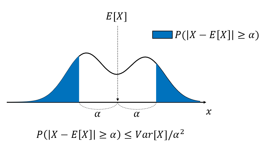
Figure 2. The Chebyshev inequality describes the probability that a random variable $x$ deviates from the extreme values $E[X]\pm\alpha$ based on the expected value of the entire data distribution.

The proof is surprisingly simple and is based on the above Markov inequality. The inequality $|X-E[X]|\gt\alpha$ in Equation (8) can be thought of as follows:

\[|X-E[X]|\geq\alpha \Leftrightarrow (X-E[X])^2\geq \alpha^2\]

Let us define a new random variable $Y$ as follows:

\[Y=(X-E[X])^2\]

Then, by definition of variance, we have $E[Y]=Var[X]$. Therefore, the Markov inequality for $Y$ and $\alpha^2$ yields:

\[P(Y\gt\alpha^2)\leq E[Y]/\alpha^2\]

Substituting back to $X$, we obtain:

\[P((X-E[X])^2\geq\alpha^2)\leq Var[X]/\alpha^2 % Equation (12)\]

Using Equation (9), we can obtain Equation (8).

Significance of Chebyshev Inequality

Let us substitute $k\sigma$ for $\alpha$ in Equation (8), where $\sigma$ denotes the standard deviation. Then we can transform Equation (8) as follows:

\[Equation (8) \Rightarrow P(\left|X-E[X]\right|\geq k\sigma)\leq Var[X]/{k^2\sigma^2} % Equation (13)\] \[\Rightarrow P(\left|X-E[X]\right|\geq k\sigma)\leq \frac{1}{k^2} % Equation (14)\]

What insight can we gain from Equation (14)? It tells us about the information that can be obtained through the mean and variance of any probability distribution. In other words, it means that almost all data in any distribution are close to the mean, and it tells us how far away they are based on the standard deviation.

Assuming that you are a professional math blogger, I will translate the sentences without summarizing or omitting any of them. Please keep the links in Markdown format as expressed as .

When $k=2$, equation (14) indicates that 25% of data lies beyond $\pm 2$ standard deviations from the expected value $E[X]$ of the probability distribution of the random variable $X$. In other words, 75% of the data lies within $\pm$ 2 standard deviations from the mean. (Note that for a normal distribution, 95% of the data falls within $\pm$ 2 standard deviations from the mean. It is worth noting that Chebyshev’s inequality is a “loose” condition that holds for any type of distribution.)

Generally speaking, Chebyshev’s inequality implies that no more than $1/k^2$ of the data falls beyond $k$ standard deviations from the mean.

Perhaps for this reason, statisticians may use the mean and standard deviation as the most useful representative values for probability distributions. By providing only the mean and standard deviation, it is possible to roughly estimate that:

“Most of the data falls within the range of the mean $\pm$ 2 standard deviations.”

without examining the overall distribution of the data.

Reference

• Outlier Analysis 2nd e.d., Charu C. Aggarwal, Springer
• The Power of Statistics that Rules Big Data (Practical Use Edition), Nishiuchi Hiromu, Vision Korea