What Eigenvalues and Eigenvectors Ask:
"When a vector x undergoes a linear transformation A, what vector remains parallel to the original vector x but only changes in magnitude?"
"Then, how much did the magnitude change?"
What Does it Mean to Perform Matrix Operations on Vectors?
A matrix is an operation of linear transformation. The term ‘linear’ may sound complicated, so let’s just call it a transformation. What does it transform? A matrix transforms a vector into another vector1.
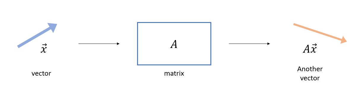
Figure 1. A matrix is an operator that transforms a vector.
As we can see from Figure 1, when a vector is transformed using a matrix, the resulting vector ($A\vec{x}$) can change in both magnitude and direction compared to the original vector ($\vec{x}$). Let’s use the applet below to explore the results of linear transformations using arbitrary vectors and matrices.
Meaning of Eigenvalues and Eigenvectors
As shown in Figure 1 and the applet above, when a vector undergoes matrix operations, it can result in a different vector than the original. However, for certain vectors and matrices, the linear transformation may only change the magnitude of the vector without changing its direction2. For example, in the above applet, if we input the vector
\[\left[\begin{array}{c} 1\\ 1\end{array}\right] \notag\]and the matrix
\[\left[\begin{array}{c} 2 & 1\\ 1 & 2\end{array}\right] \notag\]and check the result, we can see that the output vector is parallel to the input vector but with a different magnitude.
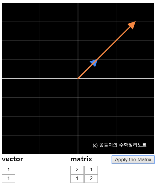
Figure 2. Some vectors and matrices output vectors that are parallel to the input vector but with a different magnitude.
In other words, the result of linearly transforming the input vector $\vec{x}$ with matrix $A$ can be expressed as a scalar multiple of the input vector.
\[A\vec{x} = \lambda \vec{x}\]
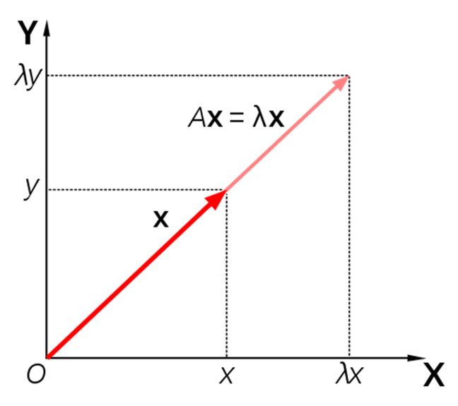
Figure 3. Some vectors and matrices output vectors that are parallel to the input vector but with a different magnitude.
Definition of Eigenvalues and Eigenvectors
| DEFINITION 1. Definition of Eigenvalues and Eigenvectors |
|---|
$$A\vec{x}=\lambda \vec{x}$$ The solution vector $\vec{x}$ is the corresponding eigenvector for eigenvalue $\lambda$. |
In this case, equation (2) can be rewritten by the properties of matrices as follows.
\[(A-\lambda I)\vec{x}=0\]Here, $I$ is the identity matrix.
There are two conditions for equation (3) to hold, which are when the expression inside the parentheses becomes 0, and when $\vec{x} = 0$. If only the first condition is met, we can find an appropriate $\lambda$ and a non-zero $\vec{x}$. However, if the second condition is satisfied, we obtain a ‘trivial solution’ with $\lambda$ and $\vec{x} =0$.
Therefore, in order to avoid obtaining the ‘trivial solution’ of $\vec{x}=0$ from the expression inside the parentheses of equation (3), the necessary and sufficient condition for having nontrivial solutions is
\[det(A-\lambda I)=0\]Calculating Eigenvectors and Eigenvalues through an Example
Let’s consider the following matrix $A$:
\[A = \left[\begin{array}{c} 2 & 1\\ 1 & 2\end{array}\right]\]We will now find the eigenvalues and eigenvectors for this matrix.
According to the definition of eigenvalues and eigenvectors, the eigenvalue $\lambda$ and eigenvector $\vec{x}$ satisfy the following equation:
\[A\vec{x} = \lambda\vec{x}\]Therefore, by the properties of matrices, we have $(A-\lambda I)\vec{x}=0$. Moreover, in order for $\vec{x}$ to have nontrivial solutions, the following condition must be satisfied.
\[det(A-\lambda I) = 0\]Hence,
\[det(A-\lambda I) = det \left( \left[\begin{array}{c} 2 - \lambda& 1\\ 1 & 2 -\lambda\end{array}\right] \right) = 0\] \[\Rightarrow (2-\lambda)^2-1\] \[= (4-4\lambda + \lambda ^2)-1\] \[=\lambda ^2 -4\lambda + 3 = 0\]Therefore, $\lambda_1=1$ and $\lambda_2=3$.
In other words, the eigenvalues of the linear transformation $A$ are 1 and 3. This means that when a vector that does not change in direction but only scales in size is transformed, its size will be multiplied by 1 and 3, respectively. Now, let’s find the eigenvectors.
Again, Equation (2) must satisfy both eigenvalues $\lambda_1=1$ and $\lambda_2=3$. Therefore, for the case of $\lambda_1=1$,
\[A\vec{x} = \lambda_1 \vec{x}\] \[\Rightarrow \left[\begin{array}{c} 2 & 1\\ 1 & 2\end{array}\right] \left[\begin{array}{c} x_1\\ x_2\end{array}\right] = 1\left[\begin{array}{c} x_1\\ x_2\end{array}\right]\]must be satisfied, which leads to the following system of linear equations:
\[2x_1+x_2=x_1\] \[x_1+2x_2=x_2\]Therefore, the eigenvector for $\lambda_1=1$ is
\[\left[\begin{array}{c} x_1\\ x_2\end{array}\right]= \left[\begin{array}{c} 1\\ -1\end{array}\right]\]Similarly, using the same method, the eigenvector for $\lambda_2=3$ is
\[\left[\begin{array}{c} x_1\\ x_2\end{array}\right]= \left[\begin{array}{c} 1\\ 1\end{array}\right]\]Geometrically, this means that the vector $\vec{x} = [1,1]$ remains unchanged in direction but scales by a factor of 3 under the linear transformation $A$. Similarly, the vector $\vec{x} = [1, -1]$ remains unchanged in direction but scales by a factor of 1 under the linear transformation $A$.