What does singular value decomposition (SVD) say: For a set of orthogonal vectors, what is the orthogonal set that can still be orthogonal after linear transformation, even though their size changes?
And what is the result of linear transformation?

※ Singular value decomposition (SVD) is usually defined for complex spaces, but this page specifies that it is written only for real vector spaces.

※ This article follows the column vector convention.

Definition of singular value decomposition

Singular value decomposition (SVD) is one of the ‘matrix decomposition’ methods that can decompose any $m\times n$ dimensional matrix $A$ as follows.

\[A = U \Sigma V^T\]

Here, the size (or dimension) and properties of the four matrices ($A, U, \Sigma, V$) are as follows.

$A$: $m\times n$ rectangular matrix
$U$: $m\times m$ orthogonal matrix
$\Sigma$: $m\times n$ diagonal matrix
$V$: $n\times n$ orthogonal matrix

---

To provide some supplementary explanations here, orthogonal matrix and diagonal matrix have the following properties.

An orthogonal matrix is a matrix that satisfies the following properties:

If $U$ is an orthogonal matrix, then

\[UU^T=U^TU=I\]

As a result, it is also verified as an additional fact that $U^{-1}=U^T$.

---

Additionally, a diagonal matrix is a matrix that satisfies the following properties.

If $\Sigma$ is a diagonal matrix, then all the values of the elements, except for the diagonal entries of $\Sigma$, are 0.

In other words, if $\Sigma$ is a $2 \times 2$ matrix, it approximately has the following form:

\[\begin{pmatrix} \sigma_1 & 0 \\ 0 & \sigma_2 \end{pmatrix}\]

Furthermore, if $\Sigma$ is an $m \times n$ matrix where $m > n$, it approximately has the following form:

\[\begin{pmatrix} \sigma_1 & 0 & \cdots & 0 \\ 0 & \sigma_2 & \cdots & 0 \\ {} & {}& \ddots & {} \\ 0 & 0 & \cdots & \sigma_n \\ 0 & 0 & \cdots & 0 \\ \vdots & \vdots & \vdots & \vdots \\ 0 & 0 & \cdots & 0 \end{pmatrix}\]

Moreover, if $\Sigma$ is an $m \times n$ matrix where $m < n$, it approximately has the following form:

\[\begin{pmatrix} \sigma_1 & 0 & \cdots & 0 &0 & \cdots & 0 \\ 0 & \sigma_2 & \cdots & 0 & 0 & \cdots & 0\\ {} & {}& \ddots & {} & {} & {} & {}\\ 0 & 0 & \cdots & \sigma_m & 0 & \cdots & 0 \end{pmatrix}\]

Geometric Interpretation of Singular Value Decomposition (SVD):

Singular value decomposition has the following meaning.

$\Rightarrow$ For a set of orthogonal vectors, what set of orthogonal vectors remains after a linear transformation that preserves their magnitudes? And what are the results of the linear transformation?

In 2-dimensional vector space…

To simplify the explanation and provide a visual understanding, let’s consider the case where matrix $A$ is $2 \times 2$ dimensional.

In a 2-dimensional real vector space, given any vector, we can always find another vector that is orthogonal to it.

A more formalized method could be using the Gram-Schmidt process to find orthogonal vectors more systematically.

However, when the same linear transformation A is applied to two orthogonal vectors, it cannot be guaranteed that they will remain orthogonal after the transformation.

The figure below shows the result of linearly transforming an arbitrary vector $\vec x$ using the matrix A:

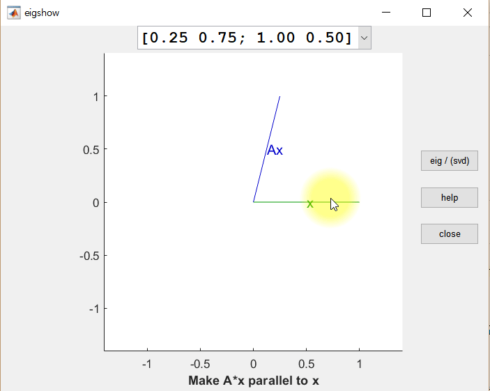
Figure 1. The result of linearly transforming an arbitrary vector x using a matrix A

Now, let’s consider what happens when we simultaneously apply linear transformations to two orthogonal vectors. Can we find cases where the result of the linear transformation is still orthogonal? The figure below shows the results of linearly transforming two orthogonal vectors $\vec x$ and $\vec y$ using the same matrix $A$ (i.e., $A\vec x$ and $A\vec y$, respectively).

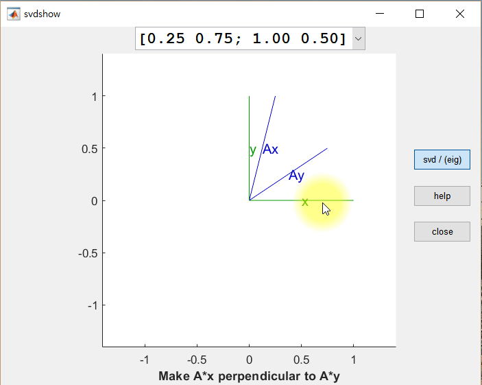
Figure 2. The results of linearly transforming an arbitrary vector x, a vector y orthogonal to x, and the results of transforming x and y using A

There are two notable observations from the above figure. First, it can be seen that $A\vec x$ and $A\vec y$ do not become orthogonal to each other in just one case.

Second, when $A\vec x$ and $A\vec y$ are transformed through the matrix $A$ (i.e., the linear transformation), their lengths change slightly. These values can be referred to as scaling factors, but generally, they are called singular values and are denoted as $\sigma_1, \sigma_2, \cdots$, with larger values being referred to first.

Going back to the beginning, an arbitrary $m \times n$ matrix $A$ can be decomposed as follows:

\[A = U\Sigma V^T\]

The orthogonal vectors $\vec x$ and $\vec y$ before the linear transformation shown in the example can be thought of as a collection of column vectors, which correspond to the $V$ matrix in the decomposition $A = U\Sigma V^T$.

\[V= \begin{pmatrix} | & | \\\\ \vec x & \vec y \\\\ | & | \end{pmatrix}\]

Additionally, if we normalize the orthogonal vectors $A\vec x$ and $A\vec y$ with unit length and call them $\vec u_1$ and $\vec u_2$, respectively, then the collection of these column vectors corresponds to the $U$ matrix in the SVD decomposition $A=U\Sigma V^T$:

\[U= \begin{pmatrix} | & | \\\\ \vec u_1 & \vec u_2 \\\\ | & | \end{pmatrix}\]

Finally, the singular values (i.e., scaling factors) can be thought of as a matrix $\Sigma$ in the following form:

\[\Sigma= \begin{pmatrix} \sigma_1 & 0 \\\\ 0 & \sigma_2 \end{pmatrix}\]

From the perspective of linear transformations, the relationship between the four matrices ($A, V, \Sigma, U$) can be expressed as follows:

\[AV=U\Sigma\]

In other words, “When the column vectors in $V$ ($\vec x$ or $\vec y$) are linearly transformed by matrix $A$, their magnitudes change by $\sigma_1$ and $\sigma_2$, respectively, but can we still find orthogonal vectors $\vec u_1$ and $\vec u_2$?”

Then, since $V$ is an orthogonal matrix, we have $V^{-1}=V^T$, and the relationship can be rewritten as:

\[AV=U\Sigma\] \[AVV^T=U\Sigma V^T\] \[A=U\Sigma V^T\]

This is the relationship that holds in SVD decomposition.

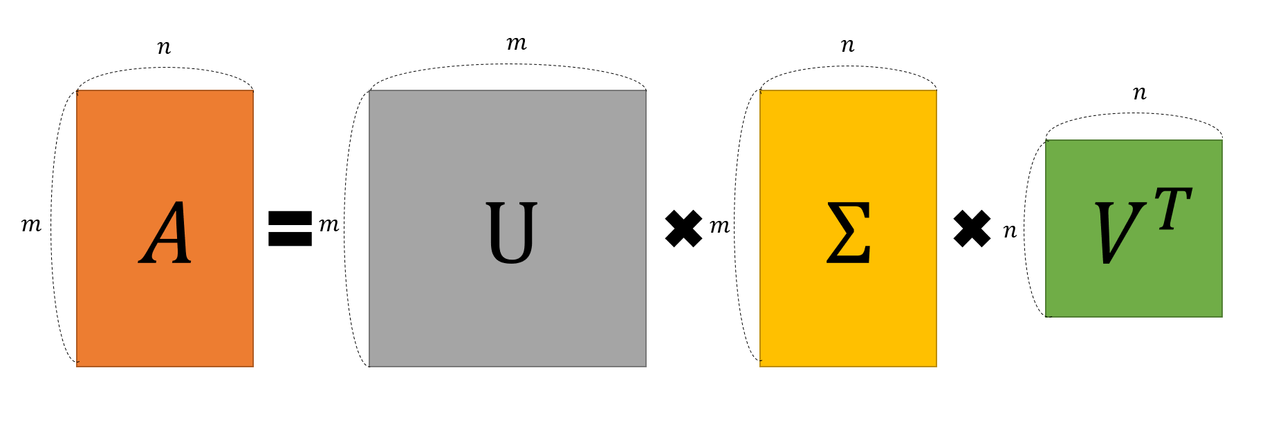
Figure 3. Visualization of the SVD decomposition of an arbitrary matrix A.

What if the input-output dimensions are different in a transformation?

When defining singular value decomposition, we stated that the matrix $A$ being decomposed is of size $m\times n$.

In other words, even if it is not a square matrix, matrix $A$ can still be decomposed.

---

It is easy to understand when we consider cases where the dimensionality decreases.

Let’s say our matrix $A$ is a $2\times 3$ matrix that reduces the dimensionality from 3D to 2D.

Then, if we reconsider what singular value decomposition (SVD) requires, we can ask if it is possible to make two vectors orthogonal even after linearly transforming them from a 3D space to a 2D space.

Let’s take a look at the animated figure below, which represents a linear transformation from 3D vector space to 2D vector space (i.e., a plane)¹.

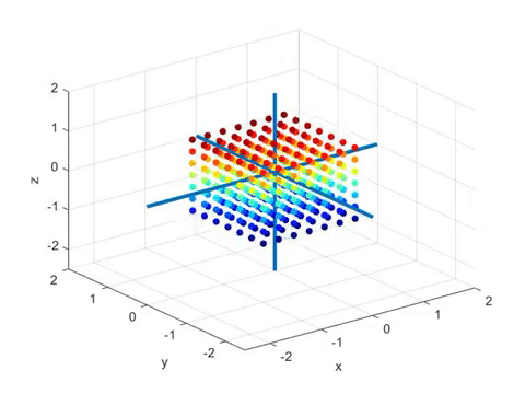
Let’s provide some additional explanation about the animation. The colored spheres represent vectors in 3D space.

Usually, arrows are used to represent vectors, but in this case, only the heads are shown as spheres.

The transformation shown in this animation is a projection of 3D vectors onto a plane.

In this case, the vectors orthogonal before and after the linear transformation through SVD can be visualized as follows.

In the last part of the video, we can see the following:

Figure 4. Results of linear transformation for a 2 x 3 matrix and the column vectors of U matrix (blue) and the row vectors of V matrix (green)

The green arrows in the figure represent the orthogonal vectors before the linear transformation, while the blue arrows represent the orthogonal vectors after the linear transformation.

This shows that even in cases where the dimensions of the input and output vectors are different due to a change in dimensionality during linear transformation, singular value decomposition can still be applied by setting one of the scaling factors (i.e., singular values) to 0.

Purpose of Singular Value Decomposition

The formula of SVD can also be described as follows.

\[A = U\Sigma V^T\] \[= \begin{pmatrix} | & | & {} & | \\\\ \vec u_1 & \vec u_2 &\cdots &\vec u_m \\\\ | & | & {} &| \end{pmatrix} \begin{pmatrix} \sigma_1 & & & & 0\\\\ & \sigma_2 & & & 0\\\\ & & \ddots & & 0\\\\ & & & \sigma_m & 0 \end{pmatrix} \begin{pmatrix} - & \vec v^T_1 & - \\\\ - & \vec v^T_2 & - \\\\ &\vdots& \\\\ - & \vec v^T_n & - \end{pmatrix}\] \[= \sigma_1 \vec u_1 \vec v_1^T + \sigma_2 \vec u_2 \vec v_2^T +\cdots+ \sigma_m \vec u_m \vec v_m^T\]

In the equation $\vec u_1 \vec v_1^T$, etc., become $m \times n$ matrices. Also, $\vec u$ and $\vec v$ are normalized vectors, so the values of the elements in $\vec u_1 \vec v_1^T$ are between -1 and 1.

Therefore, considering only the part $\sigma_1 \vec u_1 \vec v_1^T$, the size of this matrix is determined by the value of $\sigma_1$.

In other words, we can use the SVD method to decompose an arbitrary matrix A into multiple matrices of the same size as A, and the magnitudes of the values of the elements in each decomposed matrix are determined by the magnitudes of the values of $\sigma$.

In other words, SVD allows us to divide an arbitrary matrix A into multiple layers based on the amount of information it contains.

Applications of Singular Value Decomposition

The utility of singular value decomposition shines not in the process of decomposition itself, but in the process of recombining the decomposed matrices.

Using only a few of the largest singular values, we can ‘partially restore’ the original matrix A into a new matrix A’. As mentioned before, the magnitude of the singular values determines the amount of information in A, so even with a few large singular values, we can still retain useful information.

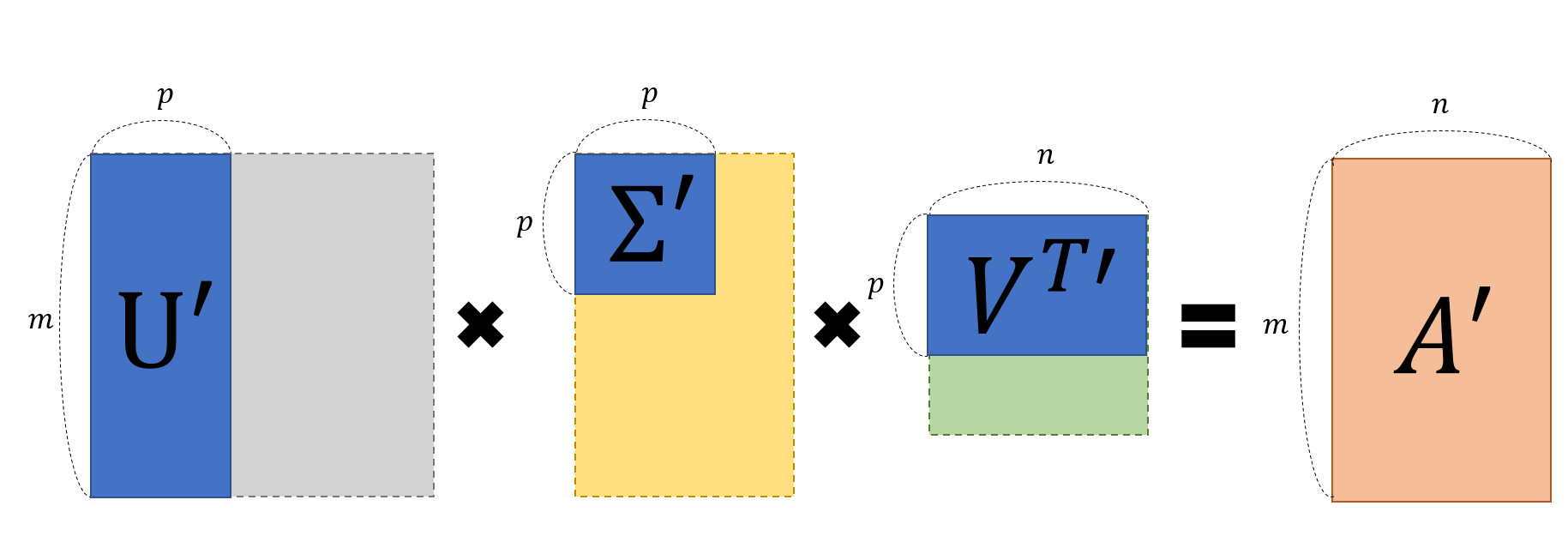
Figure 5. Partial restoration of A using only a subset of U, Sigma, V matrices obtained through singular value decomposition

In the example below, you can see the process of ‘partial restoration’ through a photo. By selectively restoring only the important information, the file size of the photo may decrease, but the intended content of the photo can still be preserved.