Jackknife & Bootstrap

Prerequisites

To better understand this post, it is recommended to know about the following topics:

Estimators and Standard Error

Meaning of Estimators

To understand the Jackknife and Bootstrap methods, it is essential to understand what an estimator is.

An estimator can be defined as a function calculated using samples.

(Whoever translated this seems to have translated ‘량’ as ‘quantity’, which seems incorrect. It would be more appropriate to translate it as estimation method, estimator or estimation function.)

For example, a function that calculates the mean or variance can be considered an estimator.

The mean value is calculated as follows. For $n$ samples $x_1, x_2, \cdots, x_n$,

\[m(X)=\frac{1}{n}\sum_{i=1}^{n}x_i\]

$m(\cdot)$ is a type of function that takes $x_1, x_2, \cdots, x_n$ as input and performs a predetermined calculation.

In this context, an arbitrary estimator can be defined.

Let’s call the estimator that I arbitrarily defined $\phi_n$. Since it is similar to defining a function, let’s easily define anything.

\[\phi_n(X)=\frac{3}{2}\sum_{i=1}^{n}\log(x_i)\]

Also, an estimator does not necessarily have to have only one output value. There are also estimators with two output values. In such cases, it is called an interval estimator, and the confidence interval estimator is representative.

Meaning of Standard Error

On the other hand, in the Meaning of Sample and Standard Error section, we discussed the standard error of the mean.

Here, the mean refers to the sample mean, and almost all the data we deal with are samples extracted from the population.

And the estimators used are also applied to the sample.

Once again, the reason for thinking about the standard error of the sample is that a sample is a subset extracted from the population.

Again, let’s consider the distribution of the height of aliens living on Venus among 150 people, with an easier example.

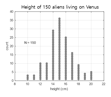
Figure 1. Distribution of the height of 150 aliens living on Venus, which is a population in imagination

Suppose we randomly select six aliens from Venus. Each time we do this, the distribution of the sample will be different, and the estimate (such as the mean, standard deviation) will also be different.

In Figure 2 below, we have conducted a sample extraction three times and drawn the sample distribution obtained each time.

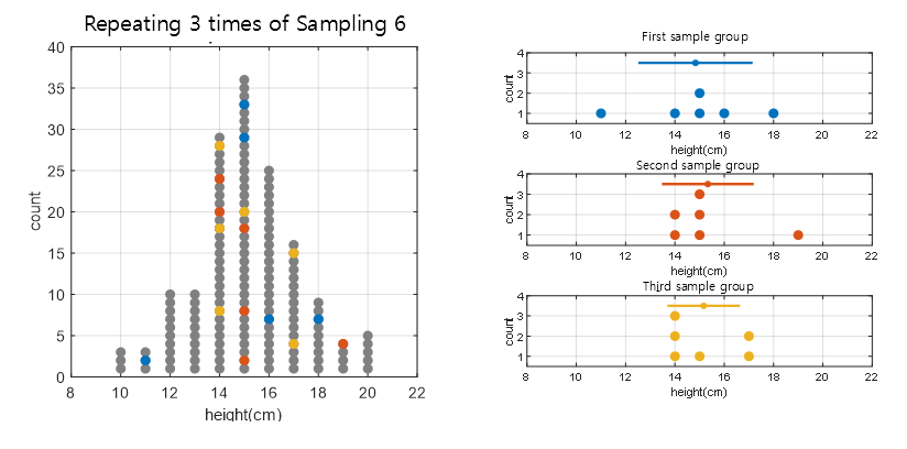
Figure 2. Drawn the sample distribution obtained each time by extracting samples three times.

What we are curious about is how the error of the estimator $\phi_n$ (i.e., the standard deviation of the estimate) is calculated.

In other words, how $std(\phi_n)$ is calculated is precisely the standard error of this estimator.

The standard error of the sample mean is well established theoretically.

However, is there a clever way to calculate the standard error of even poorly established estimators?

The Jackknife method and the Bootstrap method are ways to calculate the standard error of estimators, even those that are not well established theoretically.

Both methods use a non-parametric approach to calculate the standard error of the estimator and are based on resampling, so let’s understand both methods together.

Jackknife Method

Origin of Jackknife Method

The jackknife method is a technique developed by Quenouille and Tukey between 1949-1956.

The name “jackknife” was given to this method because it handles data in a way that resembles the actual shape of a jackknife.

Figure 3. The shape of a jackknife.

The jackknife method is a resampling-based method, which constructs a new dataset by taking one data point at a time from the given dataset.

For example, if we have a dataset (a,b,c,d), the jackknife method generates four new datasets:

(b,c,d)
(a,c,d)
(a,b,d)
(a,b,c)

This method resembles the action of removing one blade at a time from a jackknife.

The reason for constructing new datasets by taking one data point at a time is to estimate the range of error of an estimator by resampling with the available data.

In other words, the jackknife method works by taking parts of the data one by one to estimate the range of an estimator’s output¹.

This allows us to estimate the overall range of error of a device.

How to use the Jackknife Method

So, what is the specific usage of the Jackknife method?

First, let’s define some terms.

For any estimator $\phi$, $\phi_n(X)=\phi_n(X_1, \cdots, X_n)$ is an estimated value defined for the sample $X=\lbrace X_1, X_2, \cdots, X_n \rbrace$.

The subscript $n$ is used to emphasize that this is an estimate for $n$ samples.

Let $X_{[i]}$ denote the set of $n$ samples $X$ with the $i$th sample excluded.

Now, let’s consider the following value for the estimator $\phi$ on which the Jackknife method will be applied.

\[ps_i(X)=n\phi_n(X)-(n-1)\phi_{n-1}(X_{[i]})\]

The value of $ps$ is derived from the difference between the estimated value obtained using all data and that obtained by excluding the $i$th sample.

In other words, the pseudo-value shows how much the $i$th data affects the estimated value obtained using all data.

Then, the mean of $ps_i(X)$ is

\[ps(X)=\frac{1}{n}\sum_{i=1}^{n}ps_i(X)\]

and the variance is

\[V_{ps}(X)=\frac{1}{n-1}\sum_{i=1}^{n}(ps_i(X)-ps(X))^2\]

If we consider $ps_i(X)$ as independent samples, then the 95% confidence interval of the sample mean $ps(X)$ can be calculated as

\[\left(ps(X)-1.96\sqrt{\frac{1}{n}V_{ps}(X)}, ps(X)+1.96\sqrt{\frac{1}{n}V_{ps}(X)}\right)\]

Also, if we define the z-value as follows, we can determine the p-value. Let the null hypothesis be $H_0: \theta =\theta_0$. Then,

\[Z=\frac{\sqrt{n}(ps(X)-\theta_0)}{\sqrt{V_{ps}(X)}}=\frac{ps(X)-\theta_0}{\sqrt{(1/n)V_{ps}(X)}}\]

Example of using jackknife

Imagine yourself as a professional math blogger and please just translate the sentences.

Consider the following 16 data:

\[17.23,\ 13.93,\ 15.78,\ 14.91,\ 18.21,\ 14.28,\ 18.83,\ 13.45 \\ 18.71,\ 18.81,\ 11.29,\ 13.39,\ 11.57,\ 10.94,\ 15.52,\ 15.25\]

Let’s assume the following estimator:

\[\phi_n(X_1, \cdots,X_n)=\log(s^2)=\log\left(\frac{1}{n-1}\sum_{i=1}^{n}(X_i-\bar{X})^2\right)\]

If we calculate $\phi_n(X)$ using all 16 data, we can find out that

\[\phi_n(X)= 1.9701\]

(where log is natural logarithm)

If we calculate $\phi_{n-1}(X_{[i]})$ excluding each data for each data, we get the following:

\[1.994,\ 2.025,\ 2.035,\ 2.039,\ 1.940,\ 2.032,\ 1.893,\ 2.011 \\ 1.903,\ 1.895,\ 1.881,\ 2.009,\ 1.905,\ 1.848,\ 2.038,\ 2.039\]

Now, if we calculate $ps_i(X)=n\phi_n(X)-(n-1)\phi_{n-1}(X_{[i]})$, we get:

\[1.605,\ 1.151,\ 0.998,\ 0.942,\ 2.416,\ 1.043,\ 3.122,\ 1.362\\ 2.972,\ 3.097,\ 3.308,\ 1.393,\ 2.951,\ 3.806,\ 0.958,\ 0.937\]

If we calculate the mean and variance of $ps_i(X)$, we get:

\[ps(X)=2.00389\] \[V_{ps}(X)=1.0909\]

Therefore, the 95% confidence interval is $(1.4920, 2.5156)$. In fact, these 16 data are sampled from a distribution with a variance of 5.0, so we can say that the case where the true parameter is included in the confidence interval.

Bootstrap Method

The Bootstrap method is a variation of the Jackknife method, invented by Bradley Efron in 1979.

The word “bootstrap” means “self-made” or “self-reliant”. The term comes from the fact that computer booting is a form of bootstrapping, which means starting up a computer without any external help.

The English word “bootstrap” originates from the strap on the back of boots used for pulling them on. The word has a strange etymology, as it is said to have originated from the story of Baron Munchausen, who pulled himself out of a swamp by his bootstraps, although most versions of the story describe him using his hair instead.

Figure 4. The physical meaning of bootstrap

In any case, it is sufficient to know only a little about why bootstrap got its name.

Figure 5. Baron Munchausen pulling himself out of the swamp by his bootstraps. There are versions of the story that say he used his hair instead.

Overview

Bootstrap is a technique used to estimate the range of errors in an estimator, similar to the Jackknife method.

To do this, Bootstrap performs resampling, similar to the Jackknife method, but with the difference that it allows for duplicate samples. This slight difference may not seem like much, but ultimately it results in many more possible cases of resampling, and thus, more resampled samples. This leads to smoother histograms when examining resampled data.

However, dealing with many possible cases without computer assistance would be difficult. Therefore, with the development of computer technology, Bootstrap has become a practical method used today.

How to Use Bootstrap Method

The usage of bootstrap is similar to jackknife, where both methods use resampling to estimate the error range of an estimator.

However, there are two differences between them. One is that bootstrap allows for repeated sampling during resampling, and the other is that bootstrap uses the extracted data directly for the estimator without using pseudo values.

To explain it more visually, let’s say we have seven samples as shown in the figure below. (The numbers on the circles indicate the sample numbers.)

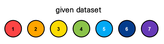
Figure 6. Seven given data samples considered to explain the usage of bootstrap

Let’s assume that we randomly resample the data with repeated extractions using these seven data samples.

For example, we can obtain the results as shown in Figure 7 below.

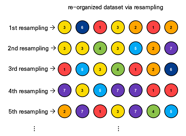
Figure 7. Seven given data samples considered to explain the usage of bootstrap

In Figure 7, resampling was only performed up to the fifth time, but if we perform resampling up to the 1000th or 5000th time, we can obtain 1000 or 5000 datasets, respectively.

By calculating the estimator value for each resampled dataset and constructing a histogram, we can estimate the error range of the estimator for each iteration.

Example of Using Bootstrap

We will reuse the dataset and estimator used in the jackknife example problem to consider the error range using the bootstrap method using Equations (8) and (9).

First, collect the datasets using resampling with 5000 duplicates allowed for the 16 datasets in Equation (8), and apply the estimator in Equation (9) to obtain 5000 estimator values. Then, plot a histogram of the 5000 estimator values obtained by applying the estimator to the bootstrap datasets.

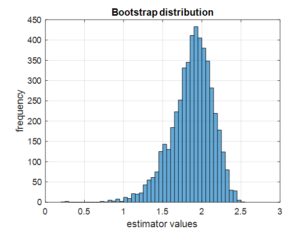
Figure 8. Histogram of estimator values obtained by applying the estimator to 5000 bootstrap datasets.

Next, sort the 5000 estimator values and find the values at the 2.5th and 97.5th percentiles, and display them. Also, since the datasets in Equation (8) are obtained from data with variance 5, we know that the true estimator value is $\log(5)=1.6094$, so let’s display the true estimator value as well. The resulting plot is shown below.

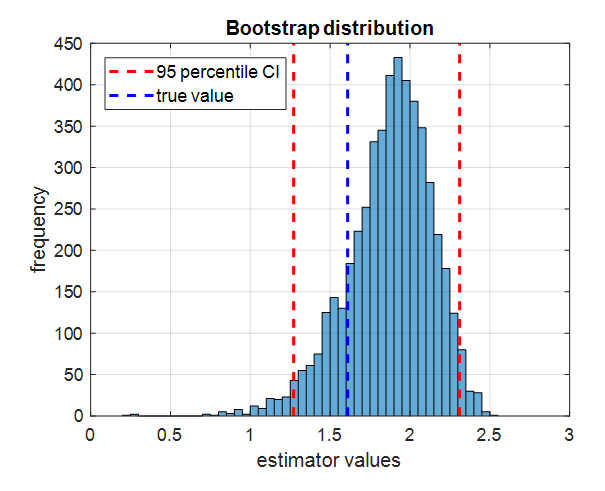
Figure 9. 95% confidence interval obtained by taking the 2.5th and 97.5th percentile values of the estimator values obtained by applying the estimator to the bootstrap datasets, along with the true value.

The 2.5th and 97.5th percentile values obtained in this way constitute a 95% confidence interval. This method is called the percentile confidence interval method and is the most intuitively understandable method.

Of course, there are other methods for calculating confidence intervals using the bootstrap method, so it is recommended to refer to the literature, such as (Singh and Xie).

In any case, the important point to note here is that the true value can fall within this 95% confidence interval.

The Significance of Bootstrap

The significance of bootstrap is that it allows us to logically estimate what the distribution of estimator values of samples that we couldn’t sample multiple times would have been like. This is covered in conjunction with the meaning of sample and standard error in Sample and Standard Error, and for estimators like the mean where the standard error is well known, there is no reason to use methods like bootstrap. However, for estimators like formula (9) where the method for calculating the standard error is not well known, bootstrap allows us to easily consider the range of errors.

References

There is also a jackknife method that removes two or three data points at a time. ↩

PREVIOUSWilcoxon Signed Sum Test

NEXTPermutation Test)