※ The content of this post is largely borrowed from Thomas Judson’s The ordinary differential equations project

So far, discussions on differential equations have mainly focused on first-order differential equations.

Moreover, in the case of a first-order, single-variable differential equation, the “order” refers to the number of variables that the differential coefficient is calculated with respect to. For example, if $t$ is the independent variable and $x$ is the dependent variable, a general equation is as follows:

\[\frac{dx}{dt}=f(t, x) % Equation (1)\]

However, differential equations are not limited to cases where there is only one dependent variable. By using two differential equations together, it is possible to model changes in two or more dependent variables simultaneously.

For example, by using the following system of equations, we can model changes in two dependent variables at the same time:

\[\begin{cases} \dfrac{dx}{dt} = f(x, y) \\\\ \dfrac{dy}{dt} = g(x, y)\end{cases} % Equation (2)\]

Predator-Prey Equations (Lotka-Volterra Equations)

A balanced food chain is a very important factor in maintaining an ecosystem.

While it may seem sad to see rabbits being eaten by foxes, if the foxes don’t eat and survive, who knows what will happen in nature.

In addition, the act of foxes eating rabbits plays a very important role in maintaining the population of rabbits.

If rabbits were left alone without any predators, their population would increase infinitely due to the lack of natural predators.

(We will investigate the issue of population saturation due to the limit of land or food using the revised Predator-Prey Equations later.)

We want to transfer the above content into a differential equation model.

This famous modeling equation is called the Predator-Prey Equations or the Lotka-Volterra Equations.

First, let’s create an equation for the population of rabbits (i.e., the prey).

Let $R$ be the population of rabbits. Initially, the population of rabbits will grow exponentially if left alone.

As we saw in part 1 of Modeling Phenomena with Differential Equations, we can apply a population growth model here.

In other words,

\[\frac{dR}{dt}=a R % 식 (3)\]

where $a>0$.

The additional content in equation (3) is the interaction between prey and predator, where some individuals of the rabbit population decrease due to the interaction with the fox population.

In other words, when they encounter a fox, they can be caught and eaten. Therefore, we can slightly modify equation (3) to derive an equation for the rabbit population as follows:

If we denote the fox population as $F$,

\[Equation(3) \Rightarrow \frac{dR}{dt} = aR -bRF % Equation (4)\]

where $a, b>0$. Also, $RF$ represents the interaction between the rabbit and fox populations, which is their product.

Now let’s try to set up an equation for the time variation of the fox population.

Let’s assume that the fox population naturally decreases if left alone. They cannot survive by eating only grass.

In other words,

\[\frac{dF}{dt}= -cF % Equation (5)\]

where $c>0$.

Furthermore, if we incorporate the factor of the interaction between the fox and rabbit created, equation (6) will be modified as follows.

\[Equation(5) \Rightarrow \frac{dF}{dt}=-cF + dFR % Equation (6)\]

Here, $c, d>0$, and $FR$ is the product of the fox and rabbit populations.

By using equations (4) and (6) together, we can confirm the balance between the populations of rabbits and foxes.

\[\begin{cases} \dfrac{dR}{dt} = aR -bRF \\\\ \dfrac{dF}{dt} = -cF + dFR\end{cases} % Equation (7)\]

There is still no known method to obtain an exact solution in a closed form of equation (7)¹².

However, what is more important to us right now is how the form of this solution works and whether the modeling of equation (7) reflects the phenomenon well.

Let’s set $a=2, b=1, c=5,$ and $d=1$ in equation (7) and draw the solution curves for the predator and prey. The initial values for both predator and prey are set to 1.

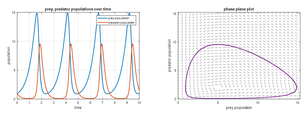
Figure 1. One of the solution curves for the predator-prey model.

Looking at the left of Figure 1, the prey (blue) grows rapidly relative to the predator (red) at first because there are few prey for the predator to eat. Thus, many predator individuals die of natural causes. However, as the prey reproduces sufficiently, more prey become available for the predator to eat, so the number of predator individuals increases.

Around time = 2, when the number of predators has become too large, the number of prey begins to decrease, presumably because more of them are being killed and eaten by predators.

On the right of Figure 1, the relationship between predator and prey is shown on the xy-plane. Starting from the point (1,1), which is the initial value, we can see the purple curve being drawn as we follow the arrows. Initially, only the number of prey increases, but as the number of predators gradually increases, the number of prey decreases.

The predator-prey model shows how the number of individuals of predator and prey change over time.

A predator-prey model with a finite carrying capacity

Let’s take a look at a modified version of the predator-prey model we saw earlier, which includes a finite carrying capacity.

This content is directly borrowed from the context of logistic growth we saw in modeling phenomena with differential equations.

In other words, in this model, the amount of grass that rabbits can eat is limited. If rabbits grow in a meadow with a limited amount of grass, which is not infinitely wide, their growth rate cannot help but be limited.

Let’s modify the equation for rabbit population growth in equation (7) using the logistic growth equation.

\[Equation (7)\Rightarrow \begin{cases} \dfrac{dR}{dt} = aR(1-\dfrac{R}{N}) -bRF \\\\ \dfrac{dF}{dt} = -cF + dFR\end{cases} % Equation (8)\]

Here, $N$ is the carrying capacity.

As in the previous analysis, let’s set $a=2, b= 1, c = 5, d = 1$, and $N=10$. When we draw the solution curve for this case, it looks like the following:

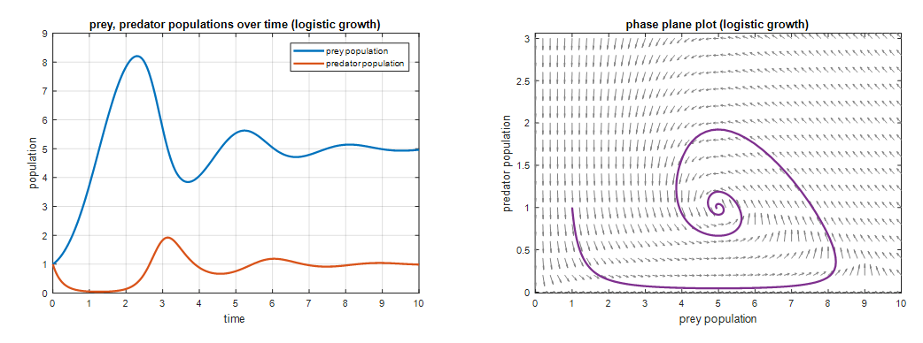
Figure 2. One of the solution curves for a predator-prey model with a finite carrying capacity

Looking at the left side of Figure 2, we can see that each population size converges to a certain value.

This can be seen more clearly in the phase plot on the right side of Figure 2, where we can see that the value converges to a ratio of about 5:1, where the ratio of prey to predator is approximately 5:1.

Moreover, as we can see from the right side of Figure 2, in a predator-prey model with a finite carrying capacity, the population size converges to a 5:1 ratio from any initial condition in the vicinity of the 5:1 ratio.

Let’s take a look at damped harmonic motion, which was one of the topics we saw in modeling phenomena with differential equations using the perspective of a system of differential equations.

The equation for damped harmonic motion was as follows:

\[m\frac{d^2x}{dt^2}+b\frac{dx}{dt}+kx = 0\]

Although this equation is a second-order differential equation, it can be rewritten as a system of two first-order differential equations as follows.

Let’s define a new variable $v$ as follows.

\[v = \frac{dx}{dt}\]

Then, the derivative of $v$ is

\[\frac{dv}{dt}=\frac{d^2x}{dt^2}=-\frac{b}{m}v-kx\]

On the other hand, what we want to see is something similar to equation (7), which means that the left-hand side should involve the derivative of two variables, and the right-hand side should involve expressions of two variables.

That is, if we let $x’$ and $v’$ denote the derivatives of $x$ and $v$, respectively, we can model it as follows.

\[\begin{cases} \dfrac{dx}{dt} = v \\ \\ \dfrac{dv}{dt} = -\dfrac{b}{m}v-kx\end{cases}\]

Here, with $b/m=0.4$ and $k=1.04$, and initial values of $x=0$ and $x’=2$, the solution curve and phase plane are shown in the following figure.

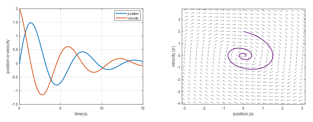
Figure 3. Solution curve and phase plane of damped harmonic motion (underdamped)

If we represent the change in position over time in the phase plane as a vibrating animation, we can also see it as follows.

Figure 4. Phase plane and vibrating motion animation of damped harmonic motion (underdamped)

As we can see from the animation above, the vibrating motion slows down gradually, but it is not damped as strongly as the force of harmonic motion, and it can be considered as a modeling of the case where it gradually slows down while repeating several periods.