Optimization Method with Momentum - ADAM

This post is a summary of Professor Andrew Ng’s lecture and discusses the use of the ADAM optimizer in deep learning training algorithms, instead of Gradient Descent, which is recommended in many tutorials using Python libraries.

We will explore why ADAM is recommended over Gradient Descent in most literature and what advantages it offers.

Prerequisites

To understand this post, it is recommended to have knowledge of the following:

Gradient Descent

The Problem with Gradient Descent

When using Gradient Descent to minimize a cost function (or error), the convergence rate can sometimes be very slow.

In some cases, increasing the step size (or learning rate) can speed up convergence, but in other cases, slow convergence occurs due to the nature of the cost function, which causes oscillation around certain parameters, as shown in Figure 1 below. In such cases, it is often necessary to wait, even if the learning rate is slow, as improper adjustments can cause the cost function to diverge.

(In Figure 1, the parameter “b” is oscillating and gradually converging to the minimum value.)

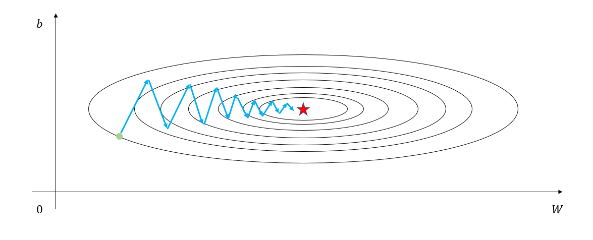
Figure 1. Convergence around a specific parameter while minimizing the cost function

The reason why oscillations occur in the cost function is that the concept of gradient itself creates a vector in a direction perpendicular to the contour line.

Therefore, considering this characteristic, what we want to achieve can be summarized as converging slowly in the vertical direction and quickly in the horizontal direction, as shown in Figure 1.

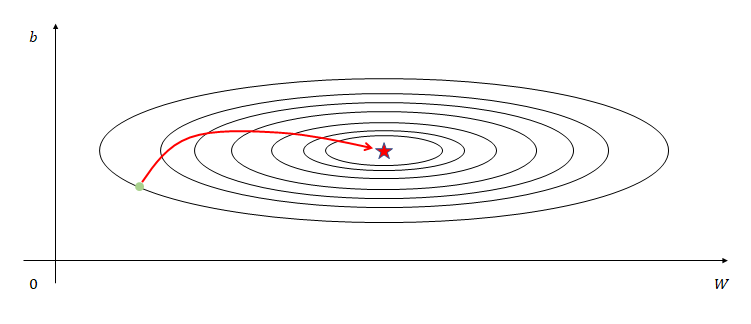
Figure 2. The desired convergence path

Gradient Descent with Momentum

The Gradient Descent with Momentum, which introduces the concept of momentum, can be described as an update method that gradually reduces the amount of change in the direction of updating when the path taken during iterations keeps changing direction, and adds acceleration when the direction is maintained.

This method is called Momentum, and let’s first look at the algorithm through pseudo-code.

Assume that the model has two parameters, $W$ and $b$, and the subscript $(t)$ indicates that it was calculated in the $t$th iteration.

[Momentum Algorithm]

Initialize $V_{dw(0)} = \vec 0$, $V_{db(0)} = \vec 0$

(Here, the dimensions of $V_{dw(0)}$ and $V_{db(0)}$ are the same as those of $W$ and $b$, respectively.)

At the $t$th iteration:

$\quad$ Calculate $dW_{(t)}$ and $db_{(t)}$ for the current batch.

$\quad$ Then, calculate the following terms.

\[V_{dw(t)} =\beta_1 V_{dw(t-1)} + (1-\beta_1)dW_{(t)}\] \[V_{db(t)} = \beta_1 V_{db(t-1)} + (1-\beta_1)db_{(t)}\]

Weight and bias update:

\[W := W - \alpha V_{dw(t)}\] \[b:= b - \alpha V_{db(t)}\]

(where $\alpha$ is the learning rate.)

The core of the Momentum algorithm is Equations (1) and (2), which have almost identical forms. Let’s expand Equation (1) a bit more by examining each iteration from the beginning.

Equation (1) is a recursively calculated term, and if we examine it carefully from iteration 1, it will be as follows:

\[V_{dw(1)} = \beta_1 V_{dw(0)} + (1-\beta_1)dW_{(1)}\]

In the second iteration,

\[V_{dw(2)} = \beta_1 V_{dw(1)} + (1-\beta_1)dW_{(2)}\] \[=\beta_1(\beta_1 V_{dw(0)}+(1-\beta_1)dW_{(1)})+ (1-\beta_1)dW_{(2)}\] \[=\beta_1^2V_{dw(0)}+ \beta_1(1-\beta_1)dW_{(1)}+(1-\beta_1)dW_{(2)}\]

In the third iteration, it goes like below.

\[V_{dw(3)} = \beta_1 V_{dw(2)}+ (1-\beta_1)dW_{(3)}\] \[= \beta_1 \left\lbrace\beta_1^2V_{dw(0)}+ \beta_1(1-\beta_1)dW_{(1)}+(1-\beta_1)dW_{(2)}\right\rbrace+ (1-\beta_1)dW_{(3)}\] \[=\beta_1^3V_{dw(0)}+ \beta_1^2(1-\beta_1)dW_{(1)}+\beta_1(1-\beta_1)dW_{(2)}+(1-\beta_1)dW_{(3)}\]

Generalizing the discussion above, we can think of what’s going to be happening in $k$th iteration.

\[V_{dw(k)} = \beta_1^k V_{dw(0)}+\beta_1^{k-1}(1-\beta_1) V_{dw(1)}+\beta_1^{k-2}(1-\beta_1) V_{dw(2)}+\cdots +\beta_1^0(1-\beta_1)V_{dw(k)}\] \[=\beta_1^kV_{dw(0)}+\sum_{i=1}^{k}\beta_1^{k-i}(1-\beta_1)V_{dw(i)}\]

Since $V_{dw(0)}$ is initialized as 0 usually, we can get the following result.

\[Equation(13) \Rightarrow \sum_{i=1}^{k}\beta_1^{k-i}(1-\beta_1)V_{dw(i)}\]

It’s common to set $\beta_1$ to around 0.9 for Momentum.

Now, let’s take another look at equation (11) to rethink the meaning of Momentum.

Looking at equation (11), we see that the current velocity $V_{dw(3)}$ is influenced by past velocities. The older the velocity relative to the current iteration, the more it is multiplied by $\beta_1$, meaning recent velocity values have a greater impact.

In other words, if the progression of the Gradient were like in Figure 1, the b-axis gradient factors that go up and down would cancel each other out and the speed would gradually approach zero, while the W-axis gradient factors that continue to move to the right would continue to add up, causing the speed to increase gradually as if inertia were at play.

RMSProp

RMSProp, short for Root Mean Square Propagation, is an algorithm proposed by Geoffrey Hinton. It’s famous for being one of the first algorithms proposed during his Coursera lecture series, and has since become a well-established algorithm, although it has not been formally published as an academic paper.

RMSProp is similar to the Gradient with Momentum method, but instead of using the direction of the gradient, it adjusts the learning rate for each parameter based on its magnitude.

Let’s take a look at the RMSProp algorithm.

[RMSProp algorithm]

Initialize $S_{dw(t)} = \vec{0}$, $S_{db(t)} = \vec{0}$

(Here, $S_{dw(0)}$ has the same dimensions as $W$, and $S_{db(0)}$ has the same dimensions as $b$.)

On iteration $t$:

$\quad$ Calculate $dW_{(t)}$ and $db_{(t)}$ for the current batch.

$\quad$ Then, calculate the following terms.

\[S_{dw(t)} =\beta_2 S_{dw(t-1)} + (1-\beta_2)dW_{(t)}^2\] \[S_{db(t)} = \beta_2 S_{db(t-1)} + (1-\beta_2)db_{(t)}^2\]

Weight and bias updates:

\[W := W - \alpha \frac{dW_{(t)}}{\sqrt{S_{dw(t)}}+\epsilon}\] \[b:= b - \alpha \frac{db_{(t)}}{\sqrt{S_{db(t)}}+\epsilon}\]

(Here, $\epsilon$ is a very small positive value less than 1 that is used to prevent division by zero when $S$ becomes very small.)

The difference between the Momentum algorithm and the RMSProp algorithm lies in the term $S_dw$ or $S_db$.

For example, applying the RMSProp algorithm in a situation like Figure 1, we can see that the magnitude of the gradient in the $W$ direction is not large but in the $b$ direction is large as the iteration progresses.

Therefore, we can expect that $S_{dw}$ will have a small value and $S_{db}$ will have a large value.

So, the process of dividing by $S_{dw(t)}$ and $S_{db(t)}$ in Equations (17) and (18) adjusts the learning process to progress faster in the $W$ direction and slower in the $b$ direction.

In other words, the significance of RMSProp is that it can adjust the size of the learning rate appropriately for each parameter.

ADAM (Adaptive Moment Estimation)

ADAM is a combination of Gradient Descent with Momentum and RMSProp.

If you look at the algorithm for ADAM, you can understand what this means.

[ADAM Algorithm]

Initialize $V_{dw(0)} = \vec 0$, $V_{db(0)} = \vec 0$, $S_{dw(0)} = \vec{0}$, $S_{db(0)} = \vec{0}$

(Here, the dimensions of $V_{dw(0)}$ and $S_{dw(0)}$ are the same as the dimension of $W$, and the dimensions of $V_{db(0)}$ and $S_{db(0)}$ are the same as the dimension of $b$.)

In the $t$-th iteration:

$\quad$ Compute $dW$ and $db$ for the current batch.

$\quad$ Then, compute the following terms:

\[V_{dw(t)} =\beta_1 V_{dw(t-1)} + (1-\beta_1)dW_{(t)}\] \[V_{db(t)} = \beta_1 V_{db(t-1)} + (1-\beta_1)db_{(t)}\] \[S_{dw(t)} =\beta_2 S_{dw(t-1)} + (1-\beta_2)dW_{(t)}^2\] \[S_{db(t)} = \beta_2 S_{db(t-1)} + (1-\beta_2)db_{(t)}^2\]

$\quad$ Update weights and biases:

\[W := W - \alpha V_{dw(t)}/\sqrt{S_{dw(t)}+\epsilon}\] \[b:= b - \alpha V_{db(t)}/\sqrt{S_{db(t)}+\epsilon}\]

The original paper on ADAM (King & Ba, 2015) recommends the following values for $\beta_1$, $\beta_2$, and $\epsilon$:

\[\begin{cases}\beta_1: 0.9 \\ \beta_2: 0.99 \\ \epsilon: 10^{-8}\end{cases}\]

Bias Correction

The Gradient Descent with Momentum, RMSProp, and ADAM algorithms all use a type of Exponentially Weighted Moving Average (EWMA) that gradually forgets the previous values using a value of $0 < \beta < 1$. The EWMA can be generally written as follows.

Let’s call the data points as $x(t)$ and assume $v(0)=0$. Then we have the following formula:

\[v(t) := \beta v(t-1) + (1-\beta)x(t)\]

Usually, $\beta$ is a value smaller than 1, and as it approaches 1, more smoothing occurs.

Figure N. EWMA results for various values of $\beta$

From the Figure N above, we can see that if more smoothing is required, increasing the value of $\beta$ will result in a lower initial smoothing result compared to the original data points.

To correct this error, we can adjust the output $v(t)$ of each iteration using the following formula:

\[v(t) := v(t) / (1-\beta^t)\]

Here, $t$ refers to the current iteration or time.

Figure M. Before (red) and after (green) adjustment