Understanding flux is important in the context of the divergence theorem in two dimensions.
Flux can be mathematically expressed as follows:
\[\int_C\vec{F}\cdot\hat{n}ds\]Or it can be described for a closed path as follows:
\[\oint_C\vec{F}\cdot\hat{n}ds\]prerequisites
To understand flux, it is recommended to have knowledge about the following:
- Line integral of vector field
- Rotation Matrix
- Parametric equations
2D flux
Flux refers to “how much flow (inward or outward) of a vector field passes through a given curve per unit time”.
Consider the vector field shown in Figure 1 below, and two arbitrary paths.
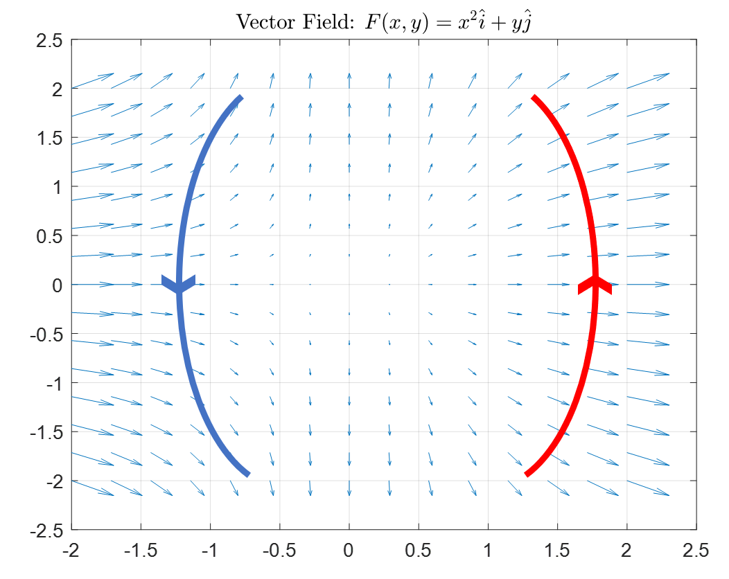
Figure 1. Given vector field F and two arbitrary paths (red and blue lines). Each path has a given direction.
If we consider the given vector field as the flow of water, then flux here refers to the total amount of water that flows in or out of the red or blue path, taking into account the direction of the vectors.
Additionally, flux can also be considered for a closed path.
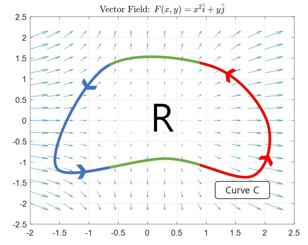
Figure 2. A given vector field F and an arbitrary closed path. The direction of the path is given.
Similar to Figure 1, we can calculate the flux over the entire path in Figure 2 for a closed path, where the portion marked in red represents the outgoing flow and the portion marked in blue represents the incoming flow.
At this point, you may be confused between flux and divergence of a vector field. To briefly explain, the divergence of a vector field represents the amount of outgoing or incoming flow in a very small area of space, while in the case of 2D flux, it represents the amount of flow exiting or entering along the path on a macro level.
Deriving the formula for 2D flux
To derive the formula for 2D flux, we will first examine the flux for a tiny path and then integrate it over the entire path.
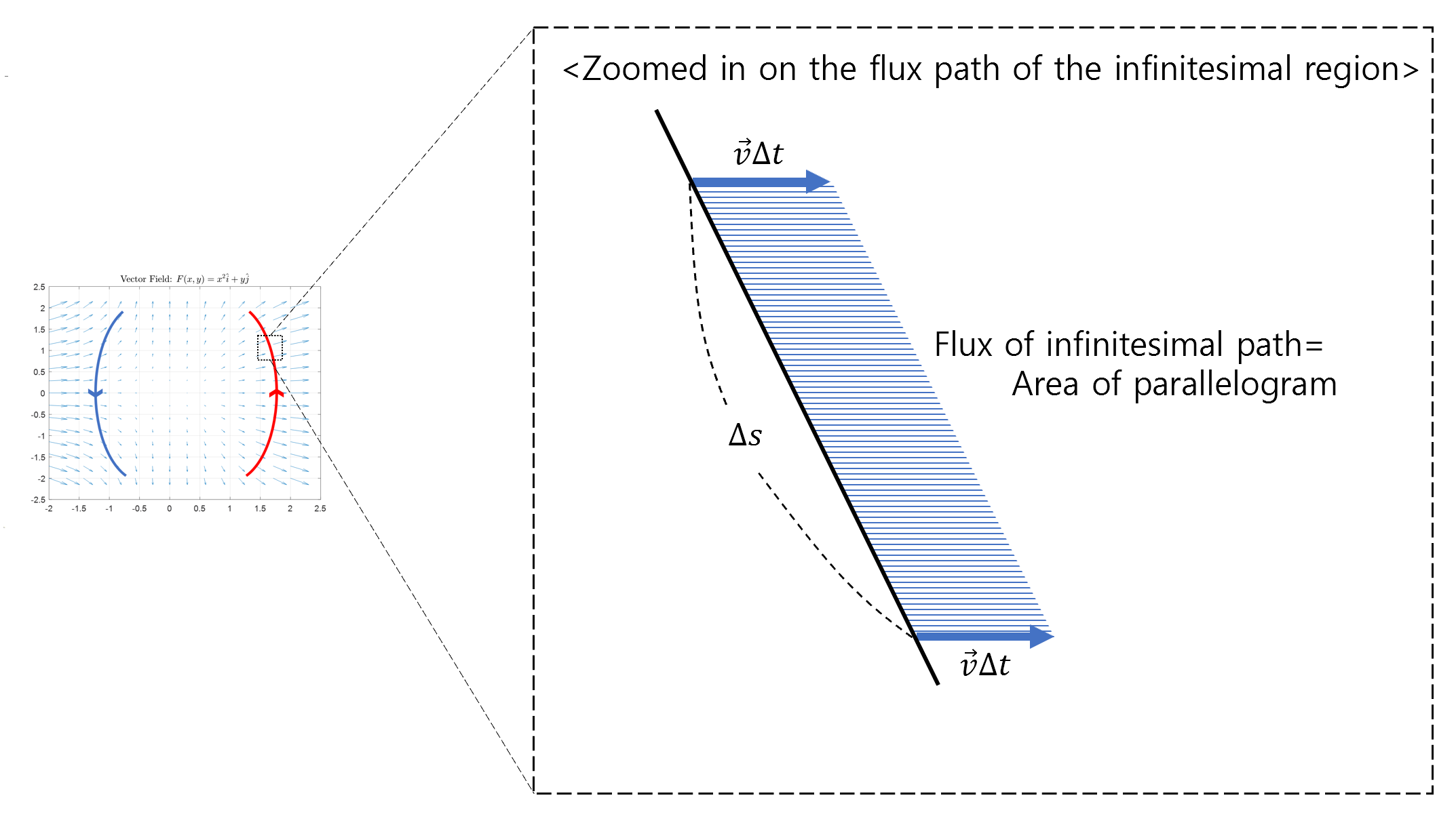
Figure 3. The flow for a tiny path. If we think of vector v as the flow rate of water, then the area of the parallelogram can be thought of as the amount of water that flows out through the tiny path in Δt time.
As seen in Figure 3, the flow for a tiny path can be obtained by calculating the area of a parallelogram. If we think of vector $\vec{v}$ as the flow rate of water and assume that this water flows for Δt time, we can calculate the amount of water that flows out through the tiny path by calculating the area of the parallelogram.
The area of the parallelogram is the product of the base and the height, where the base length is denoted by Δs and the height is obtained by taking the dot product of vector $\vec{v}\Delta t$ and the normal vector of the base.
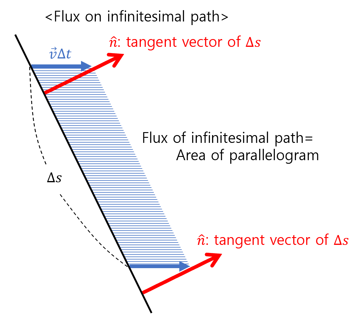
Figure 4. To calculate the area of the parallelogram, we need to multiply the base by the height. The height of the parallelogram can be obtained by taking the dot product of vector vΔt and the normal vector of Δs.
In other words, the area of a parallelogram, which is the same as the flux, can be expressed as follows:
\[flux = \Delta s(\vec{v}\Delta t \cdot \hat{n})\]The concept of flux refers to the amount of flow per unit time, so if we divide the above equation by $\Delta t$, we get:
\[flux_{\Delta s}= \Delta s(\vec{v} \cdot \hat{n})\]Ultimately, the flux for the entire path can be expressed as follows:
\[\sum flux_{\Delta s}=\sum (\vec{v} \cdot \hat{n})\Delta s\]Here, by making $\Delta s$ very small and using the symbol $\vec{F}$ to represent a general vector field instead of $\vec{v}$, we can derive the formula for flux:
\[\text{2D flux} = \int_C\vec{F}\cdot\hat{n}ds\]Generally, the direction of the normal vector ($\hat{n}$) is considered to be positive in the direction to the right along the path.
Additional steps for practical calculation of flux
While equation (6) shows that the formula for flux has been derived successfully, to actually calculate the flux, $\hat{n}$ or $ds$ must be expressed in terms of a single variable.
Usually, to represent an arbitrary path, we use parameter equations. Therefore, let’s refine the formula for flux with respect to the commonly used parameter $t$.
Calculation of the normal vector
To calculate the normal vector of the path, let’s start with the concept of a tangent vector.
Suppose a path $r$ is given by a parameter equation as follows:
\[r(t) = x(t)\hat{i} + y(t)\hat{j}\]The tangent vector represents the time derivative of a path, so it can be expressed as:
\[r'(t) = x'(t)\hat{i} + y'(t)\hat{j}\]The tangent vector $\vec{T}$ only has information about its direction without any information about its magnitude. Thus, it can be expressed as:
\[\vec{T}(t) = \frac{r'(t)}{|r'(t)|}=\frac{x'(t)\hat{i} + y'(t)\hat{j}}{\sqrt{x'(t)^2 + y'(t)^2}}\]Using the rotation matrix, we can compute the normal vector from the tangent vector. Generally, the rotation matrix for a counterclockwise rotation angle $\theta$ is given by:
\[\begin{bmatrix}\cos\theta & -\sin\theta\\\sin\theta & \cos\theta\end{bmatrix}\]As shown in the following figure, we can obtain the normal vector by rotating the tangent vector by $-90^\circ$.
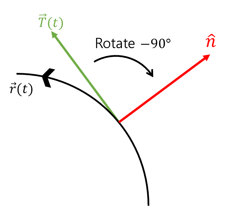
Figure 5. The relationship between the tangent vector and the normal vector
Since $\cos(-90^\circ)=0$ and $\sin(-90^\circ)=-1$, the rotation matrix is:
\[\begin{bmatrix}0 & 1\\-1 & 0\end{bmatrix}\]Therefore, for an arbitrary vector $[x, y]^T$, applying the rotation matrix yields:
\[\begin{bmatrix}0 & 1\\-1 & 0\end{bmatrix}\begin{bmatrix}x\\y\end{bmatrix}=\begin{bmatrix}y\\-x\end{bmatrix}\]In other words, to rotate a vector by $-90^\circ$, we simply need to swap its components and multiply the new $y$ component by -1.
Therefore, if we use the tangent vector, we can calculate the normal vector as follows:
\[Equation (9) \Rightarrow \frac{y'(t)\hat{i}-x'(t)\hat{j}}{\sqrt{x'(t)^2 + y'(t)^2}} = \hat{n}(t)\]Calculation of ds
$ds$ is given by the Pythagorean theorem:
\[ds = \sqrt{dx^2+dy^2}\]Using the parameter equations, we can derive:
\[ds = \sqrt{\left(\frac{dx}{dt}\right)^2 + \left(\frac{dy}{dt}\right)^2 }dt = \sqrt{x'(t)^2 +y'(t)^2}dt\]Combining the equation for the normal vector and ds
If we express the normal vector and ds as functions of the parameter $t$, we obtain the following:
\[\int_C\vec{F}\cdot\hat{n}\text{ }ds = \int_C\vec{F}\cdot \frac{y'(t)\hat{i}-x'(t)\hat{j}}{\sqrt{x'(t)^2 + y'(t)^2}} \sqrt{x'(t)^2 +y'(t)^2}dt\] \[=\int_C\vec{F}\cdot\left(\frac{dy}{dt}\hat{i}-\frac{dx}{dt}\hat{j}\right)dt\] \[=\int_C\vec{F}\cdot\left(dy\hat{i}-dx\hat{j}\right)\]Now, if we consider the vector field $\vec{F}(x,y)$, which is typically written as:
\[F(x,y) = P(x,y)\hat{i} + Q(x,y)\hat{j}\]and if $t$ varies from $a$ to $b$, we can write:
\[Equation (18) = \int_{t=a}^{t=b}Pdy-Qdx\]Example Problem
Given the vector field $\vec{F}=2\hat{i}$, calculate the flux along the line segment from $(3,0)$ to $(0,3)$.
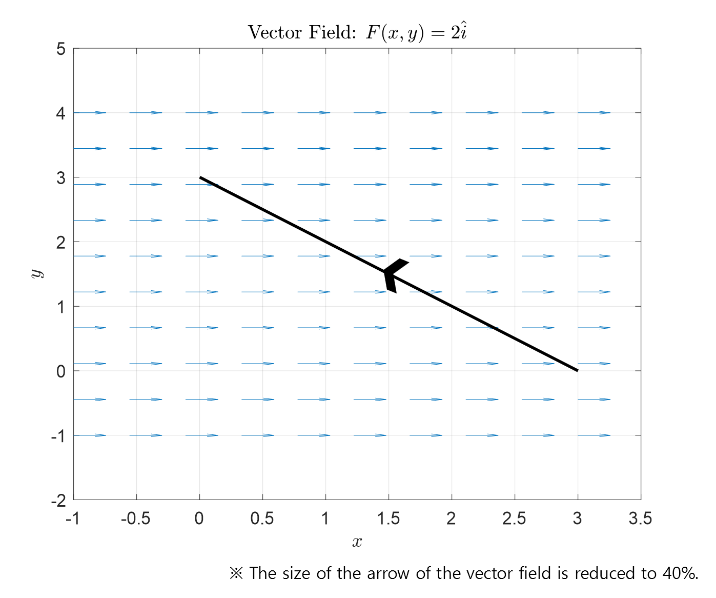
Figure 6. The given vector field and the path in the example problem.
First, let’s use parameterization to express $x(t), y(t)$:
\[\begin{bmatrix}x(t) = 3-3t\\y(t) = 3t\end{bmatrix}\text{ where }0\le t \le 1\]And,
\[\begin{bmatrix}dx = -3dt\\dy = 3 dt\end{bmatrix}\text{ where }0\le t \le 1\]The flux can be calculated as follows:
\[\int_C\vec{F}\cdot \hat{n}=\int_{t=0}^{1}Pdy-Qdx\] \[=\int_{t=0}^{1}2\cdot (3dt)-(0)(-3dt)\] \[=6\int_{t=0}^{1}dt=6\]Therefore, the flux along the line segment is 6.