In high school statistics classes, the central limit theorem is often explained as follows:

In natural or social phenomena, it is often observed that the graph of the probability density function is symmetrically distributed around a certain value and appears as a bell-shaped curve, like the one shown on the right, with the frequency decreasing as it moves away from the center.

A Korean Highschool Textbook “Probability and Statistics”, Jihaksa, 2009

The “graph on the right” referred to here is a graph of the general normal distribution.

This sentence makes you think that it would have been better if they had explained in more detail why this phenomenon occurs.

Furthermore, since the formula for the normal distribution is also complicated, it is natural for beginners to feel resistant.

\[f(x) = \frac{1}{\sigma\sqrt{2\pi}}\exp\left(-\frac{(x-\mu)^2}{2\sigma^2}\right)\]

The key keyword for the central limit theorem is “average.”

To understand the central limit theorem, it is important to understand the process of extracting the sample mean.

Let’s think about the process of extracting a sample from a population.

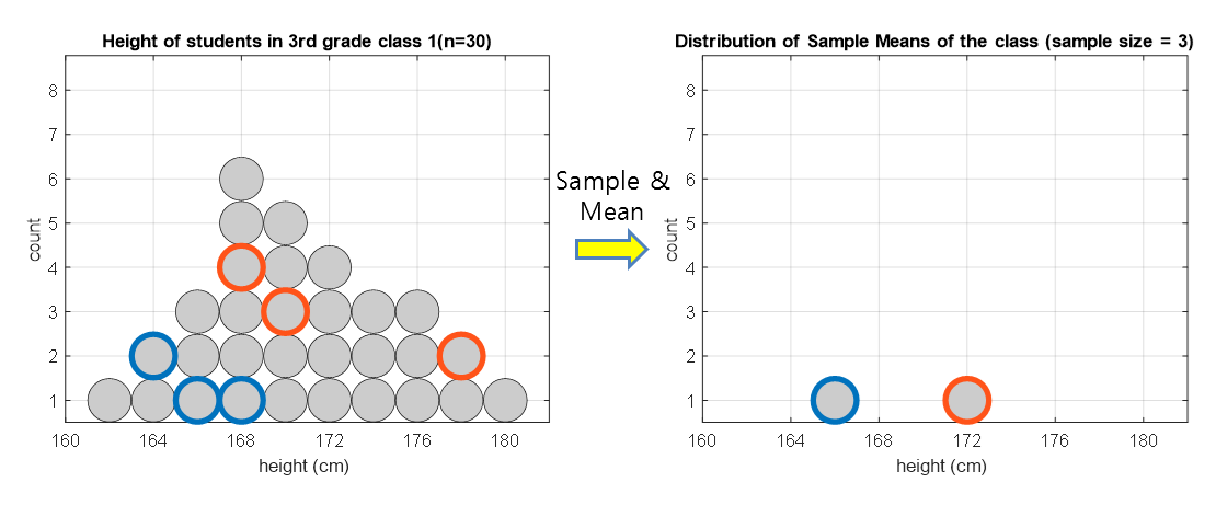
Figure 1. Histogram of the sample mean calculated by extracting a sample of size 3 from the population twice and calculating the mean each time.

Typically, when we talk about a population, we are referring to a very large group of individuals, but in this case, let’s consider a very small population to help with understanding.

Suppose we have a population consisting of all students in 3rd grade class 1 and we are interested in their height.

Extracting a sample means randomly selecting some of the 30 students from the entire population.

Also, there is one process that is necessary when extracting a sample, which is to specify the size of the sample. This is up to the researcher to decide. In the case of Figure 1, the sample size was set to 3.

As you can see on the left side of Figure 1, three students were randomly selected each time a sample was extracted.

We can then calculate the mean height of the sample and display it on the right side of Figure 1 in histogram form.

For example, the blue data in Figure 1 were extracted with three values of 164, 166, and 168, so the mean is 166.

This mean value is shown in blue as a histogram in Figure 1.

What happens if we do sample extraction infinitely many times?

In the above, sample extraction was performed only twice. However, what kind of distribution of sample means will be obtained if sample extraction is performed infinitely many times, as seen on the right side of Figure 1?

To answer this question, the distribution of sample means will converge to a normal distribution only when the sample extraction is performed infinitely many times.

(Note that as the sample size increases (i.e., the more samples taken at once), the distribution of sample means converges closer to the normal distribution.)

Increasing the number of sample extraction to 100 is merely to verify the distribution of the sample using the Monte Carlo method since it is not feasible to perform an infinite number of sample extractions in reality.

Figure 2. Histogram of the mean values of the extracted sample in each round when a sample of size 3 is extracted 100 times

Central Limit Theorem holds regardless of the shape of the population

Meanwhile, in Figures 1 and 2, the shape of the population was similar to that of a normal distribution. Is this why the distribution of the sample means follows a normal distribution?

The answer is no.

The reason why the Central Limit Theorem is powerful is that the distribution of sample means follows a normal distribution regardless of the shape of the population.

Below is an example of a histogram of sample means when the population has a distribution shape that is completely different from Figures 1 and 2.

In Figure 3 below, it is assumed that the population has a uniform distribution.

Figure 3. Histogram of the mean values of the extracted sample in each round when the population has a uniform distribution

Summary:

To summarize what we have learned, the following are true:

• The distribution of sample means approximates a normal distribution.
• Regardless of the shape of the population, the central limit theorem holds.
• Even if the samples are extracted from different populations that are independent of each other, the distribution of sample means approximates a normal distribution¹.

So why do natural or social phenomena often exhibit bell-shaped distributions, as mentioned in the textbook?

In my opinion, natural and social phenomena occur not only with individual characteristics, but also with the combination of various characteristics, resulting in an average outcome, which is why these phenomena follow a bell-shaped curve.

Moreover, another reason we focus on studying statistics with the central limit theorem is that we often compare samples based on their means, and the central limit theorem is relevant to such phenomena. As a result, we encounter many theories related to the central limit theorem.