Prerequisites
To better understand this post, it is recommended that you know about the following:
To fully understand the EM algorithm below, it is also recommended that you know about the following:
It is recommended to focus on understanding the meaning of Prior for the Naive Bayes classifier.
GMM (Gaussian Mixture Model)
[Review] Fitting a normal distribution using Maximum Likelihood Estimation
In the previous discussion of Maximum Likelihood Estimation, we learned about how to estimate parameters for given data.
In particular, we looked at fitting a normal distribution to the data as an example.
Figure 1 below shows an example of selecting an appropriate mean value among candidates using Maximum Likelihood Estimation.
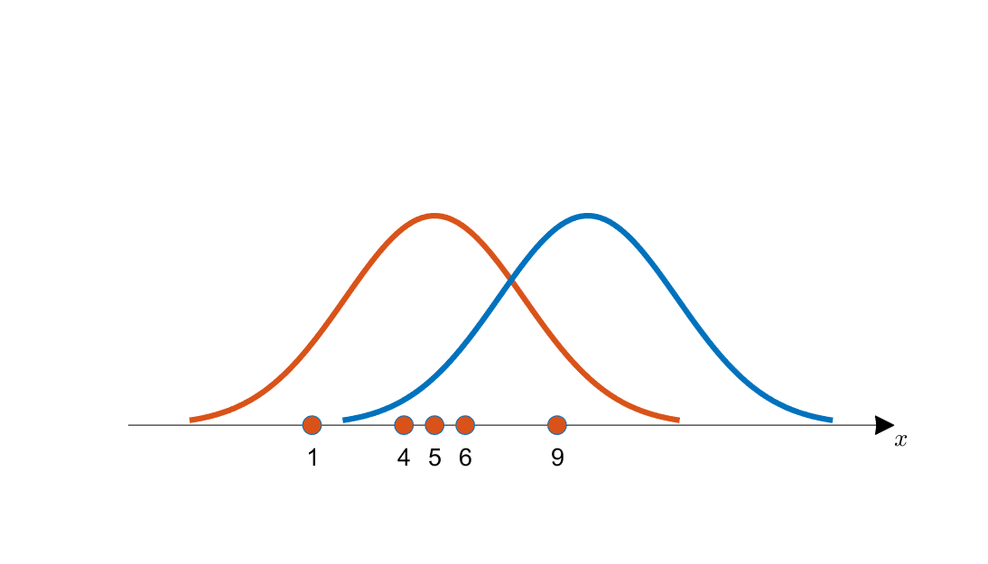
Figure 1. Obtained data and two candidate distributions for estimation (shown in orange and blue curves, respectively)
For more detailed information, it is recommended to read the Maximum Likelihood Estimation post. To briefly explain the content of Figure 1, the orange data points on the vertical axis are more likely to have come from the orange curve in Figure 1 than the blue curve. This is the essence of Maximum Likelihood Estimation.
And, assuming a normal distribution for the data, the conclusion of the maximum likelihood method for the two parameters (mean, variance) for the given $m$ data was as follows:
When we have given data $\lbrace x^{(1)}, x^{(2)}, \cdots, x^{(m)}\rbrace$, the likelihood function is maximized when calculating the mean and variance values.
\[\hat{\mu}= \frac{1}{m}\sum_{i=1}^{m}x^{(i)}\] \[\hat{\sigma}^2= \frac{1}{m}\sum_{i=1}^{m}(x^{(i)}-\mu)^2\]These results are the formulas that we are familiar with for mean and variance. However, it should be noted that this result obtained the mean and variance values that maximize the likelihood of the given data, after calculating the likelihood for the given data.
The Problem We Face and the Solution
※※※※※ Caution ※※※※※
The solution described in this section cannot be considered a complete explanation of the GMM algorithm because it only partially explains the GMM algorithm from a likelihood perspective without considering the prior $\phi$ described in the EM algorithm section below.
However, please note that the purpose of this section is to help understand the EM algorithm by understanding the overall outline of the GMM algorithm.
Nevertheless, if you are not particularly interested in the specific workings of the GMM algorithm, reading this section alone should be sufficient.
Let’s assume that there are 10 data points on a vertical line as shown in Figure 2 below.
Let’s assume that each data point has a label. (The color inside the circle represents different labels.)
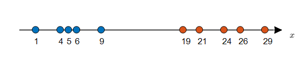
Figure 2. Density Estimation problem with given labels (can be solved using MLE)
Can we estimate the probability distribution for this dataset?
Although there are various ways to estimate the probability distribution, if we estimate the probability distribution using a parametric method, we first have to assume a distribution and estimate the parameters that fit the distribution. The maximum likelihood method (MLE) mentioned earlier is a very good way to estimate the distribution parameters for the given data. Figure 3 below can be considered as the result of estimating the probability distribution by assuming a normal distribution for the given data in Figure 2 and estimating the parameters. The parameter estimation process can be carried out by calculating the mean and standard deviation values for each label’s data using the result of MLE.
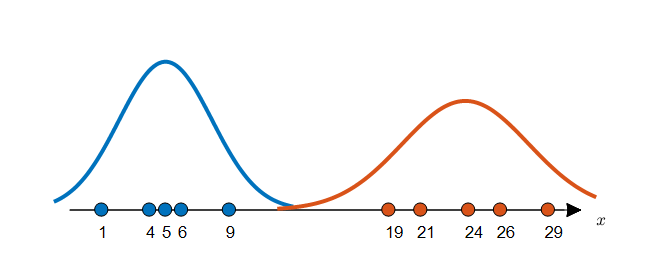
Figure 3. Two estimated distributions for labeled data.
However, what if we do not have the labels?
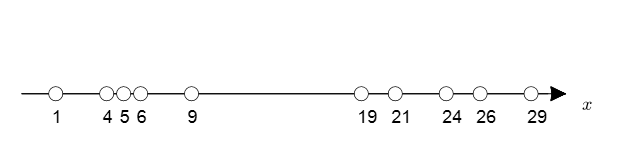
Figure 4. Distribution of unlabeled data.
Figure 4 above shows the case of unlabeled data, similar to the data in Figure 2.
To assign labels, we need a probability distribution, but to obtain a probability distribution, we need to know the parameters, and to know the parameters, we need labels for each data again.
In other words, the problem we are given is like the chicken and egg problem.
Therefore, what we can do is to randomly assign labels and start, or randomly set distributions and start, one of the two.
Let’s randomly assign distributions to each label and start.
At this time, we want to give a distribution for each label based on each parameter ($\mu, \sigma$).
If two distributions are given, we can label each data by comparing the height value (i.e., likelihood) of the distribution for each data.
Let’s say the mean and standard deviation for each group, orange and blue, are as follows:
\[\mu_1 = 3, \sigma_1 = 2.9155\] \[\mu_2 = 10, \sigma_2 = 3.9623\]Then, we can see the distribution for each label as shown in Figure 5.
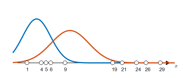
Figure 5. What if the distributions for two labels (0, 1) are given?
If a distribution similar to Figure 5 is randomly given, we can select the label for each data sample according to that distribution. Figure 6 below shows the process of selecting the label for a data sample where $x=9$.
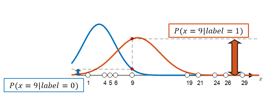
Figure 6. By using the given distribution, we can assign labels to each data sample. In this case, the label for the data corresponding to $x=9$ will be 1.
Using the method in Figure 6, we can confirm labels for all data samples, which will result in the following outcome as seen in Figure 7.
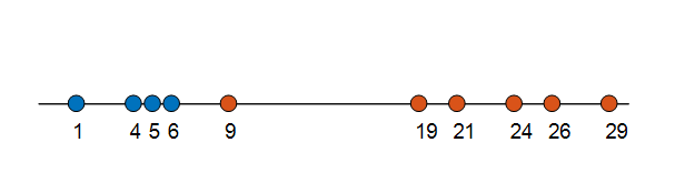
Figure 7.
Now let’s predict the distribution of each group based on the labels obtained from Figure 7.
The means and standard deviations of each group are as follows:
\[\mu_1 = 4, \sigma_1 = 2.1602\] \[\mu_2 = 21.33, \sigma_2 = 7.0048\]If we plot the distribution of each group using these values, we get the following:
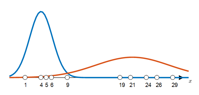
Figure 8.
Comparing Figures 5 and 8, we can clearly see that the distribution has changed.
We can then use this changed distribution to re-label the data again. If we continue this process, the distribution will eventually converge.
A summary of this process in one figure is roughly as follows:
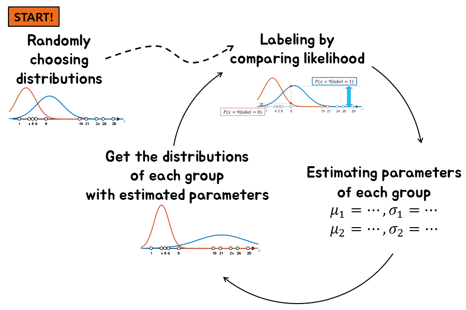
Figure 9. A method for performing clustering when labels are not given.
The result of performing these methods multiple times can be seen in the video below.
In the video below, only up to epoch = 10 was repeated, but if the distribution does not converge, the number of iterations can be increased as much as necessary.
Figure 10. Clustering process for unlabeled data using Gaussian Mixture Modeling assuming a normal distribution of the dataset
In this way, the process of performing clustering for unlabeled data assuming a normal distribution of the dataset is called Gaussian Mixture Modeling.
EM Algorithm and GMM
In the previous section, we discussed the problem we faced and its solution.
To summarize, the problem we faced was that we had unlabeled data and what we needed was the distribution for each label.
The reason why this problem is difficult is that to obtain a label, we need a distribution, and to obtain a distribution, we need a label.
To solve the problem, we assumed that the datasets would follow a normal distribution. Then, we performed clustering by giving random parameters and obtaining labels, and then obtaining distributions again using those labels.
(It is a side note that this clustering method is called Gaussian Mixture Modeling.)
This can be seen as one of the applications of the generally called EM algorithm.
The EM algorithm stands for Expectation-Maximization, where
Expectation calculates the expected value of the log-likelihood, which can be seen as the process of finding labels, and
Maximization can be seen as the process of estimating parameters using Maximum Likelihood Estimation.
That is, in the E-step, the “information of the variables (i.e., what is the label of this variable?)” is updated, and in the M-step, the “hypothesis about how the variables are distributed” is updated.
Below is the flow of the GMM algorithm from the perspective of the EM algorithm, expressed in mathematical notation.
Repeat until convergence: {
$\quad$(E-step) For each $i$, $j$, set
\[w_j^{(i)} := p(z^{(i)} = j|x^{(i)};\phi,\mu,\Sigma)\]$\quad$(M-step) Update the parameters:
\[\phi_j := \frac{1}{m}\sum_{i=1}^{m}w_j^{(i)}\] \[\mu_j := \frac{\sum_{i=1}^{m}w_j^{(i)}x^{(i)}}{\sum_{i=1}^{m}w_j^{(i)}}\] \[\Sigma_j := \frac{\sum_{i=1}^{m}w_j^{(i)}\left(x^{(i)}-\mu_j\right)\left(x^{(i)}-\mu_j\right)^T}{\sum_{i=1}^{m}w_j^{(i)}}\]}
Here, $i$ represents the order of the data, $j$ represents the label, $x^{(i)}$ represents the $i$-th dataset, and $z^{(i)}$ represents the label of the $i$-th dataset.
Also, $w_j^{(i)}$ represents the probability that the $i$-th data belongs to group $j$.
$\phi$ represents the data ratio between groups. For example, if group 0 and 1 data exist in a ratio of 6:4, then $\phi = [0.6, 0.4]$.
$\mu_j$ represents the mean value of group $j$, and $\Sigma_j$ represents the standard deviation or covariance matrix.
Although there may seem to be many complex things, let’s break them down one by one.
E-step decomposition
As explained in the GMM part, random initialization is needed to start the EM algorithm.
Looking at the (E-step) flow of the EM algorithm, the equation $w_j^{(i)} := p(z^{(i)} = j|x^{(i)};\phi,\mu,\Sigma)$ shows that we already consider $\phi, \mu, \Sigma$ as given parameters.
Regarding $\phi$, we will explain it gradually, but for now, it can be considered as the sum of weights for each label. It is okay to initialize it for each label as $[0.5, 0.5]$.
$\mu$ and $\Sigma$ are equations for mean and variance, respectively. The reason why the covariance matrix is expressed in uppercase Greek letters such as $\Sigma$ is that as the dimensionality of the input increases, the covariance must also be considered.
In other words, $\sigma$ represents the standard deviation, but $\Sigma$ represents the covariance matrix. For now, it is okay to think that $\Sigma$ is the standard deviation in one dimension.
$\mu$ and $\Sigma$ can be randomly given and initialized as shown in Figure 5.
(Let’s not consider the problem of falling into local maxima for now.)
Then, how should we interpret the equation $w_j^{(i)} := p(z^{(i)} = j|x^{(i)})$?
It means that, given the data $x^{(i)}$ and assuming the probability distribution for each label based on the parameters $\phi, \mu, \Sigma$ provided, we will calculate the probability that the $i$-th data belongs to group $j$ based on the height of that distribution.
For example, if the value $w_j^{(i)}$ indicates that there are a total of three groups and the probabilities of belonging to group 0, 1, and 2 are 0.8, 0.15, and 0.05, respectively, then:
\[w_0^{(i)} = p(z^{(i)} = 0|x^{(i)}) = 0.8\] \[w_1^{(i)} = p(z^{(i)} = 1|x^{(i)}) = 0.15\] \[w_2^{(i)} = p(z^{(i)} = 2|x^{(i)}) = 0.05\](Note that the probabilities of belonging to each group for the $i$th data point must sum to 1.)
More specific probability calculations can be performed based on Bayes’ theorem.
The equation may look complicated, but the probability that the $i$th data point belongs to group $j$ given $x^{(i)}$, $\phi$, $\mu$, and $\Sigma$ can be obtained by dividing the prior x likelihood values included in each label by the sum of all prior x likelihood values included in each label.
The equation can be written as:
\[p(z^{(i)}=j|x^{(i)};\phi,\mu,\Sigma) =\frac{p(x^{(i)}|z^{(i)} = j; \mu, \Sigma)p(z^{(i)}=j;\phi)}{p(x^{(i)};\phi, \mu, \Sigma)}\] \[= \frac{p(x^{(i)}|z^{(i)} = j; \mu, \Sigma)p(z^{(i)}=j;\phi)}{\sum_{k=1}^{l}p(x^{(i)}|z^{(i)} = k; \mu, \Sigma)p(z^{(i)}=k;\phi)}\]M-step decomposition
If you understand the E-step well, the M-step should not be difficult.
In the M-step, the $w_j^{(i)}$ values calculated in the E-step are used to estimate the parameters.
These parameters can all be easily calculated using maximum likelihood estimation. (Note that $x^{(i)}$ is given for all data points.)
As explained earlier, $\phi$ represents the data ratio between groups, $\mu_j$ represents the mean value of group $j$, and $\Sigma_j$ represents the standard deviation or covariance matrix.
However, to be precise, $\phi$ can be considered a value related to the prior probability, and $\phi$ represents the mean membership probability of each group.
For example, if there are 10 data points as shown in the figure below, $\phi$ can be calculated based on $w_j^{(i)}$.
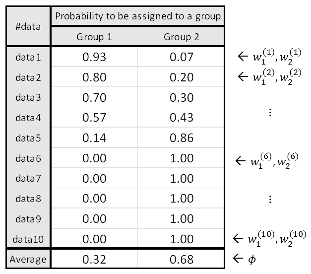
Figure 11. Calculating $\phi$ based on the given $w$
The calculation of the formula in the M-step is not difficult, but if you think it’s insufficient, you can refer to the MATLAB code below.
MATLAB code
Below is the MATLAB code for implementing the GMM algorithm in the EM algorithm perspective.
In this process, we want to create virtual data in a 7:3 ratio and give the means of 0 and 15, respectively.
It would be helpful to check the attached video when running the code at the bottom.
clear; close all; clc;
% My GMM algorithm

%% Make Synthetic Data
% I will create a virtual dataset with two groups. Mean of the groups will be 0, 15 in order to separate them as possible.
% The ratio of the number of groups will be 7:3. I.e., phi = [0.7, 0.3].

% Creating dataset
rng(1)
mu = [0, 15];
vars = [12, 3];
n_data = 1000;
phi = [0.7, 0.3];
X = [];
for i_data = 1:n_data
    if rand(1) < 0.7
        X(end+1) = randn(1) * sqrt(vars(1)) + mu(1);
    else
        X(end+1) = randn(1) * sqrt(vars(2)) + mu(2);
    end
end

% To check the distribution of data
figure('position',[628, 334, 774, 577],'color','w');
histogram(X, 50,'Normalization','pdf')

xx = linspace(-30, 30, 100);
yy1 = normpdf(xx, mu(1), sqrt(vars(1)));
yy2 = normpdf(xx, mu(2), sqrt(vars(2)));

hold on;
grid on;
plot(xx, yy1 * phi(1)+ yy2 * phi(2), 'k','linewidth',2); % 즉, phi = [0.7, 0.3]
xlabel('x');
ylabel('pdf');

%% GMM Algorithm

clear h
my_normal = @(x, mu, sigma) 1/(sigma * sqrt(2*pi)).*exp(-1 * (x-mu).^2/(2*sigma^2));

% random initialization
est_mu = [-25, 20];
est_vars = [7, 9.5];

est_w = zeros(n_data, 2);
est_phi = [0.5, 0.5];

est_yy1 = normpdf(xx, est_mu(1), sqrt(est_vars(1)));
est_yy2 = normpdf(xx, est_mu(2), sqrt(est_vars(2)));

h1 = plot(xx, est_yy1 * est_phi(1), 'r','linewidth',4);
h2 = plot(xx, est_yy2 * est_phi(2), 'g','linewidth',4);
t = text(-27, 0.075, 'the first initialization','fontsize',12);

pause;

delete(t);
delete(h1);
delete(h2);

% GMM iteration
n_iter = 50;
for i_iter = 1:n_iter

    %%%%%%%%%%%%%%%%%%%%%%%%%%% E-step %%%%%%%%%%%%%%%%%%%%%%%%%%%%%%%%%%%%
    for i_data = 1:n_data
        l1 = my_normal(X(i_data), est_mu(1), sqrt(est_vars(1)));
        l2 = my_normal(X(i_data), est_mu(2), sqrt(est_vars(2)));

        est_w(i_data, 1) = (l1 * est_phi(1)) / (l1 * est_phi(1) + l2 * est_phi(2));
        est_w(i_data, 2) = (l2 * est_phi(2)) / (l1 * est_phi(1) + l2 * est_phi(2));
    end
    %%%%%%%%%%%%%%%%%%%%%%%%%%% E-step done %%%%%%%%%%%%%%%%%%%%%%%%%%%%%%%

    %%%%%%%%%%%%%%%%%%%%%%%%%%% M-step %%%%%%%%%%%%%%%%%%%%%%%%%%%%%%%%%%%%
    % Estimating phi
    est_phi = 1/n_data * sum(est_w, 1);

    % Estimating mu
    est_mu(1) = (X * est_w(:,1))/sum(est_w(:,1));
    est_mu(2) = (X * est_w(:,2))/sum(est_w(:,2));

    % Estimating Sigma
    est_vars(1) = sum(est_w(:,1)'.*(X-est_mu(1)).^2)/sum(est_w(:,1));
    est_vars(2) = sum(est_w(:,2)'.*(X-est_mu(2)).^2)/sum(est_w(:,2));

    %%%%%%%%%%%%%%%%%%%%%%%%%%% M-step done %%%%%%%%%%%%%%%%%%%%%%%%%%%%%%%

    % Below is for visualization
    est_yy1 = normpdf(xx, est_mu(1), sqrt(est_vars(1)));
    est_yy2 = normpdf(xx, est_mu(2), sqrt(est_vars(2)));

    h1 = plot(xx, est_yy1 * est_phi(1), 'r','linewidth',4);
    h2 = plot(xx, est_yy2 * est_phi(2), 'g','linewidth',4);
    t = text(-27, 0.075,  ['Epoch: ',num2str(i_iter),' / ',num2str(n_iter)],'fontsize',12);
    pause;

    if i_iter < n_iter
        delete(t);
        delete(h1);
        delete(h2);
    end

end
Figure 11. The visualization of GMM clustering for my virtual dataset.