※ Please check this post for the proof of Shannon-Nyquist sampling theory.

Comparison of the difference between the continuous signal (white) and the restored signal by sampling (blue)

Relationship between continuous signals, discrete signals, and digital signals

These days, digital devices are ubiquitous. We use MP3 players instead of cassette tapes, coexist with paper books and e-books, and all analog TV broadcasts have been converted to digital broadcasts.

In daily life, digital devices often come with the image of “considering convenience” or “applying the latest technology.” As much research has been conducted, it can be said to be a useful technology that is closely related to real life.

The Digital Signal Processing course covers the techniques and theories needed to analyze these digital signals.

Then, how is a digital signal different from an analog signal?

As shown in the figure below, a digital signal is a digital conversion of an analog signal.

This type of converter is called an Analog-to-Digital Converter. Conversely, there is also a process of restoring from Digital to Analog. This type of converter is called a Digital-to-Analog Converter.

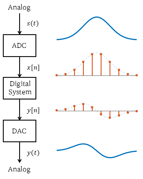
Figure 1. Digital processing system of an analog signal

If you look closely at a digital signal, you can see that the signal is received at a constant time interval. The reason for storing the signal at a fixed time interval is that the memory of digital devices is finite.

The process of storing a continuous signal at a fixed time interval is called time sampling.

Most analog signals are often real functions, and real numbers are infinite. Computers cannot accept this, so they only receive a finite number of function values.

Horizontal axis is often sampled visibly, but there are cases where the vertical axis is not paid attention to as it is also transformed into a discrete value through quantization.

Quantization theory may seem simple, but the theory is actually complex and the ideas for hardware implementation are also quite complicated. This blog will not delve deeply into quantization.

Anyway, a signal where both time sampling and quantization have been performed is finally called a “digital signal”.

In addition, a signal where only time sampling is performed is often referred to as a “discrete signal”, and it is sometimes distinguished from a digital signal depending on the presence of quantization.

Side effects of time sampling

Since any signal can be expressed as a linear combination of sinusoidal waves with different frequencies, we think about sinusoidal waves.

Moreover, since sinusoidal waves are signals that come from the movement on a circle, they have a period, and some considerations arise in sampling due to this periodicity.

A discrete sinusoidal wave coming from continuous sinusoidal waves with different frequencies

Let’s consider an arbitrary sinusoidal wave $x(t)$.

\[x(t) = A\cos(\omega_0 t)\]

If we sample this signal with a period of $T_s$, we get the following discrete signal:

\[x[n]=x(nT_s) = A\cos(\omega_0 nT_s) = A \cos(\Omega_0 n)\]

Here, $\Omega_0=\omega_0 T_s \text{[rad]}$ is the angular frequency of the discrete sinusoidal wave signal. This differs from the angular frequency $\omega_0 \text{[rad/sec]}$ of the continuous sinusoidal wave signal.

(By the way, angular frequency refers to the frequency calculated by multiplying the frequency by $2\pi$. For example, the angular frequency of a sinusoidal wave obtained from a circle rotating with a period of 1 second is $2\pi$.)

Note that $\Omega_0$ has a unit of radians and $\omega_0$ has a unit of radians per second. In other words, time information disappears in $\Omega_0$.

Therefore, if $\omega_0$ is large and $T_s$ is small, or if $\omega_0$ is small and $T_s$ is large, the discrete signal can be obtained identically even though the frequency of the continuous signal is different.

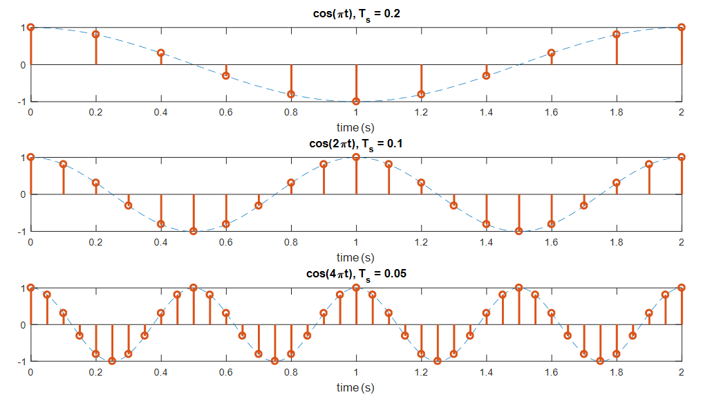
Figure 2. Even if they have different frequencies and sampling periods, they can still obtain the same discrete signal.

When sampling a sinusoidal wave with frequency $f_0+kf_s$ (where $k$ is an integer) at a sampling frequency of $f_s$, the result is the same as sampling a sinusoidal wave with frequency $f_0$.

\[\cos(2\pi(f_0+kf_s)nT_s)=\cos(2\pi f_0nT_s+2\pi knf_s T_s)\] \[=\cos(2\pi f_0 nT_s + 2\pi kn) = \cos(2\pi f_0 nT_s)\]

The problem of aliasing when restoring discrete sinusoidal waves to continuous sinusoidal waves

Looking at the above problem in reverse, it can be said that it is not always possible to restore an arbitrary discrete sinusoidal wave to the original continuous signal.

Even if we sample sinusoidal waves with different frequencies, we can get a discrete signal with the same frequency $f_0$, which is called an alias of $f_0+kf_s$ with respect to the sampling frequency $f_s$.

The phenomenon of aliasing is when the original signal cannot be distinguished during the sampling process, which results in the restoration of a different signal from the original signal¹.

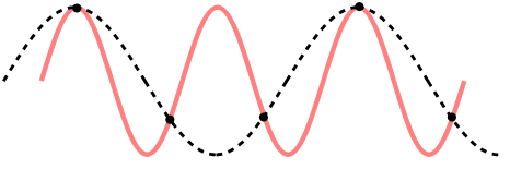
Figure 3. Aliasing phenomenon

To prevent the phenomenon of aliasing, it is necessary to sample at a sufficiently high frequency.

As can be seen from the applet at the top of this post, if we sample at a fast enough rate, which is above a certain threshold, we can reconstruct the original continuous signal from the discrete signal fairly closely.

Figure 4. To prevent aliasing, we need to sample at a sufficiently high frequency.

The Shannon-Nyquist Sampling Theorem is a theory that provides an answer to the mathematical question of “how fast do we need to sample?” However, in order to understand this theorem, one needs to have an understanding of Fourier series/transforms, which will be covered in more detail later. In short, the conclusion of the Shannon-Nyquist Sampling Theorem is that if we sample a signal at twice the frequency of its maximum frequency component, we can reconstruct the original signal.

Frequency Characteristics of Discrete Signals

If we look at the horizontal axis of a discrete signal, we can see that only the sequence number is indicated.

Since the interval between sequence numbers is always 1, the minimum period that can be used to represent this signal is 1.

In other words, the maximum frequency will be 1 and the minimum frequency will be 0.

Usually, the frequency range of a discrete signal, including negative frequencies, can be expressed as

\[-0.5 \lt F \lt 0.5\]

or

\[-\pi \lt \Omega \lt \pi\]

On the other hand, we can also consider the frequency characteristics of a discrete sinusoid.

Any signal can be expressed as a linear combination of sinusoids with different frequencies, and this applies not only to continuous signals but also to discrete signals. Therefore, when analyzing a discrete signal, it is often useful to use sinusoids.

There are some differences between discrete sinusoids and continuous sinusoids. Discrete sinusoids are not always periodic signals. In other words, depending on the sampling period, a discrete sinusoid may or may not be a periodic signal.

Let’s assume an arbitrary discrete sinusoidal signal $x[n]$ as follows:

\[x[n]=A\cos(\Omega_0 n)\]

If $x[n]$ is a periodic signal with a period of $N$, then the following must hold (where $N$ is an integer):

\[x[n]=x[N+n]\] \[\Rightarrow A\cos(\Omega_0 n) = A\cos(\Omega_0 (n+N))\]

Therefore, the digital angular frequency $\Omega_0$ must satisfy

\[\Omega_0 N = 2\pi k \Rightarrow \Omega_0 = \frac{2\pi k}{N}\]

(where $k$ is an integer),

or the digital frequency $F_0 = \Omega_0/2\pi$ must be a rational number satisfying

\[\frac{\Omega_0}{2\pi}=F_0=\frac{k}{N}\]

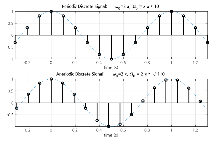
Figure 5. A discrete signal becomes a periodic signal only when the digital frequency is a rational number.

In summary, a discrete sinusoidal signal can represent all frequency components within $-\pi$ to $\pi$ and has a periodicity of $2\pi$.

Therefore, a discrete signal has a periodicity with a frequency spectrum that is copied with a period of $2\pi$ within the frequency range of the digital angular frequency $-\pi$ to $\pi$.

The following figure compares the spectrum of a periodic signal with its sampled and discretized result:

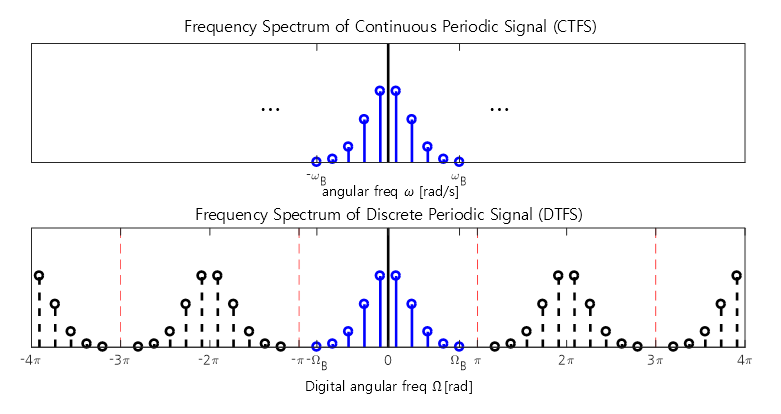
Figure 6. The frequency spectrum of a discrete periodic signal displays copies of the original continuous periodic signal at intervals of $2\pi$.

Additionally, the following figure compares the spectrum of a non-periodic signal with its discrete counterpart obtained through time sampling.

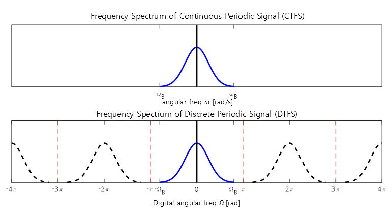
Figure 7. The frequency spectrum of a discrete non-periodic signal is a replication of the original continuous signal at intervals of $2\pi$.

References

• McClellan, James H., et al. “Signal Processing First.” Pearson Education, 2014.
• Lee, Chulhee. “Digital Signal Processing.” Hanbit Academy, 2017.