Prerequisites
To better understand this post, we recommend that you be familiar with the following:
Introduction to cyclic permutation matrix
A permutation matrix is a matrix that swaps the order of rows.
However, the permutation matrix we will use in this post performs cyclic permutation.
In other words, performing cyclic permutation on a vector $x$ means performing the following operation on the permutation matrix $P$:
\[P\vec{x} = \begin{bmatrix}x_{n-1}\\x_0\\ x_1 \\ \vdots \\ x_{n-2}\end{bmatrix}\]where
\[\vec{x} = \begin{bmatrix}x_0\\x_1\\ \vdots \\ x_{n-1}\end{bmatrix}\]To perform this operation, the cyclic permutation matrix must be defined as follows:
\[P = \begin{bmatrix} 0 & 0 & \cdots & 0 & 1 \\ 1 & 0 &\cdots & 0 & 0 \\ 0 & \ddots &\ddots & \vdots & \vdots \\ \vdots & \ddots & \ddots & 0 & 0 \\ 0 & \cdots & 0 & 1 & 0\end{bmatrix}\]In other words, the elements directly below the diagonal (subdiagonal) must have a value of 1, and the upper-right value of the matrix must be 1.
An interesting property of the cyclic permutation matrix is that if we apply $P$ twice, the rows will shift twice.
In other words,
\[P\cdot P\vec{x} = P^2\vec{x} = \begin{bmatrix}x_{n-2}\\x_{n-1}\\ x_0 \\ \vdots \\ x_{n-1}\end{bmatrix}\]Moreover, if we directly write $P^2$, it will be as follows:
\[P^2 = \begin{bmatrix} 0 & 0 & \cdots & 1 & 0 \\ 0 & 0 &\cdots & 0 & 1 \\ 1 & \ddots &\ddots & \vdots & \vdots \\ \vdots & \ddots & \ddots & 0 & 0 \\ 0 & \cdots & 1 & 0 & 0\end{bmatrix}\]To shift the rows $n$ times, we can multiply the $P$ matrix by itself $n$ times.
Decomposition of Signals (Vectors) using Cyclic Matrices
To think about the decomposition of signals (vectors), let’s first consider the discrete unit sample function, which serves as the basis for decomposing signals. Let’s use $\delta$ to denote the symbol of the discrete unit sample function.
\[\delta =\begin{bmatrix}1\\0\\ \vdots \\ 0\end{bmatrix}\]For any arbitrary vector, we can express it as a sum of scaled unit sample functions as follows:
\[\begin{bmatrix}x_0\\x_1\\ \vdots \\ x_{n-1}\end{bmatrix}= x_0 \begin{bmatrix}1\\0\\ \vdots \\ 0\end{bmatrix} + x_1 \begin{bmatrix}0\\1\\ \vdots \\ 0\end{bmatrix} + \cdots + x_{n-1} \begin{bmatrix}0\\0\\ \vdots \\ 1\end{bmatrix}\]In other words, Equation (7) asserts that any vector can be expressed as a sum of unit sample functions scaled by constants in the standard normal basis.
On the other hand, any vector $x$ in Equation (7) can also be expressed using the discrete unit sample function $\delta$ and cyclic permutation matrix $P$ as follows:
\[= x_0 \delta + x_1 P\delta + x_2P^2\delta+\cdots x_{n-1} P^{n-1}\delta\]Since $\delta = I\delta$, we can also express Equation (8) as follows:
\[Equation (8) \Rightarrow = x_0 I \delta + x_1 P\delta + x_2P^2\delta+\cdots x_{n-1} P^{n-1}\delta\] \[= \left(x_0 I + x_1 P + x_2P^2+\cdots x_{n-1} P^{n-1}\right)\delta\]From here, we can directly write the matrix expressions for $P$, $P^2$, and so on, and rewrite Equation (10) as follows:
\[\begin{bmatrix}x_0\\x_1\\ \vdots \\ x_{n-1}\end{bmatrix} = \begin{bmatrix} x_0 & x_{n-1} & \cdots & x_2 & x_1 \\ x_1 & x_1 &\cdots & x_3 & x_2 \\ x_2 & \ddots &\ddots & \vdots & \vdots \\ \vdots & \ddots & \ddots & x_0 & x_{n-1} \\ x_{n-1} & \cdots & x_2 & x_1 & x_0 \end{bmatrix} \begin{bmatrix}1\\0\\ \vdots \\ 0\end{bmatrix}\]Here, the matrix multiplied in front of $\delta$ in Equation (11) is generally called a circulant matrix.
From now on, we will denote the symbol for a circulant matrix as $C$, and Equation (11) can be generalized as follows:
\[\vec{x} = C\delta=\left(\sum_{i=0}^{n-1}x_i P^{i}\right)\delta\]Relationship between circulant matrices and discrete convolution
In signal processing theory, the Kronecker delta function is defined as follows:
\[\delta[n] = \begin{cases}1 && \text{ if }n=0 \\ 0 && \text{otherwise}\end{cases}\]
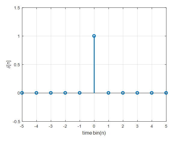
Figure 1. Kronecker delta function
Using the Kronecker delta function, we can decompose an arbitrary discrete signal as follows:
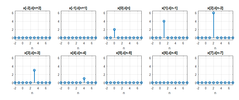
Figure 2. An arbitrary discrete function can be thought of as decomposed using the Kronecker delta function.
We can write this as a formula:
\[x[n]=\cdots + x[-2]\delta[n+2]+x[-1]\delta[n+1]+x[0]\delta[n]+x[1]\delta[n-1]+x[2]\delta[n-2]+\cdots\]Alternatively, we can write it as:
\[x[n]=\cdots + x[n+2]\delta[-2]+x[n+1]\delta[-1]+x[n]\delta[0]+x[n-1]\delta[1]+x[n-2]\delta[2]+\cdots\]Equation (15) can be written as:
\[x[n] = \sum_{k=-\infty}^{\infty}x[n-k]\delta[k]\]If we consider the equation above only for $0\leq k \leq N-1$, it can be written as follows:
\[x[n] = \sum_{k=0}^{N-1}x[n-k]\delta[k]\]Rewriting equation (16) for $0\leq n \leq N-1$, we have:
\[x[0] = x[0]\cdot 1 + x[0-1]\cdot 0 + \cdots + x[0-(N-1)]\cdot 0\] \[x[1] = x[1]\cdot 1 + x[1-1]\cdot 0 + \cdots + x[1-(N-1)]\cdot 0\] \[\vdots \notag\] \[x[N-1] = x[N-1]\cdot 1 + x[(N-1)-1]\cdot 0 + \cdots + x[(N-1)-(N-1)]\cdot 0\]Furthermore, if we combine equations (18) to (20) into a matrix form, we can write it as follows:
\[\begin{bmatrix}x[0]\\x[1]\\ \vdots \\ x[N-1]\end{bmatrix} = \begin{bmatrix} x[0] & x[N-1] & \cdots & x[1-(N-1)] & x[0-(N-1)] \\ x[1] & x[0] &\cdots & x[2-(N-1)] & x[1-(N-1)] \\ x[2] & \ddots &\ddots & \vdots & \vdots \\ \vdots & \ddots & \ddots & x[0] & x[N-1] \\ x[N-1] & \cdots & x[2] & x[1] & x[0] \end{bmatrix} \begin{bmatrix}1\\0\\ \vdots \\ 0\end{bmatrix}\]When considering this equation, if we assume that $x[n]$ is a periodic function with period $N$, then it can be viewed as a decomposition of the vector represented by a circulant matrix, as seen in equation (11).
In conclusion, using a circulant matrix to represent a vector is similar to decomposing a signal using convolution in signal processing theory.