What Fourier Series tells you: a periodic function can be represented as sum of trigonometric functions.

Prerequisites

To better understand this post, it is recommended that you have knowledge of the following topics:

• Signal Space
• Deriving Euler’s Formula with Differential Equation
• Geometrical Meaning of Euler’s Formula

An Easy Explanation of Fourier Series

Imagine there are three types of toy blocks, each with a very different shape.

Figure 1. Let's imagine toy blocks in the shape of a triangle, circle, and star.

Now, let’s say the toy blocks are all mixed up in a mess. What we want to do is to put these toy blocks into boxes based on their shapes. Is there a way to do this all at once?

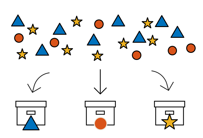
Figure 2. Is there a way to tidy up the toy blocks all at once?

Of course, it would be great if we could just magically sort them, but unfortunately, we don’t have magical powers. So how about this idea? We could use a filter that can let only the blocks of the corresponding shape pass through, and pour all the toys through it. This way, the blocks would go into the boxes that match their shapes.

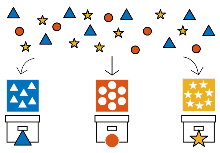
Figure 3. Having a filter that can separate the toy blocks by their shapes might make organizing them easier.

You might wonder why suddenly we’re talking about blocks and filters, but it’s because these ideas are the core concepts of Fourier series (or transformation).

Fourier series (or transformation) is a process that decomposes a signal containing multiple frequency components into individual frequency components. This process is often referred to as Fourier analysis.

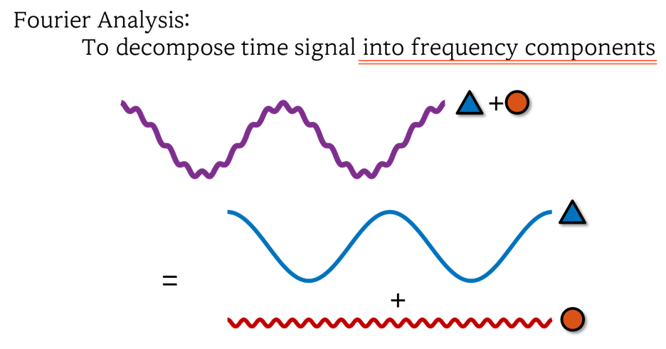
Figure 4. The essence of Fourier analysis is to decompose a signal containing multiple frequency components into individual frequency components.

The obtained frequency components are then represented on the frequency axis, rather than the time axis, and this representation is called the (frequency) spectrum.

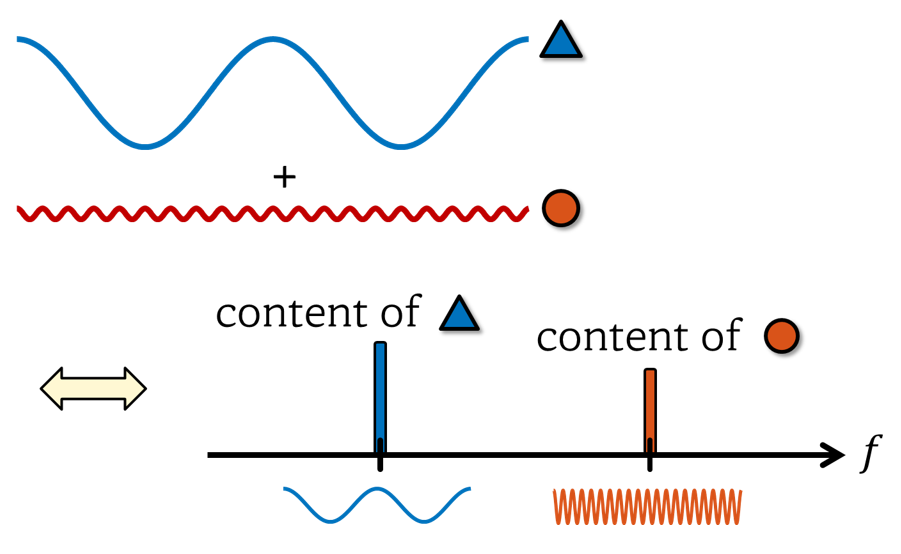
Figure 5. The essence of Fourier analysis is to decompose a signal containing multiple frequency components into individual frequency components.

When performing Fourier series, the largest period (or lowest frequency) of the periodic signal to be analyzed is determined, and the sinusoidal waves that are integer multiples of that frequency are prepared in advance.

So, using the ‘inner product’, we calculate how similar each sinusoidal wave is to the signal and examine how much each frequency component is present in the signal.

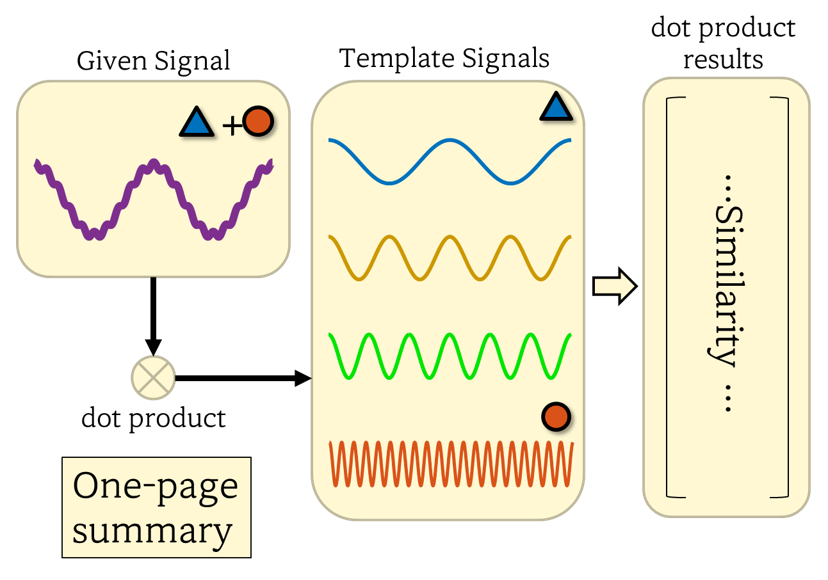
Figure 6. Fourier analysis (synthesis) can be summarized as a process of examining the frequency content of a signal by calculating inner product with pre-prepared sinusoidal waves of different frequencies.

One of the reasons why Fourier analysis is useful is that if we can analyze the signal on the frequency spectrum, it becomes easier to remove unwanted specific frequency components.

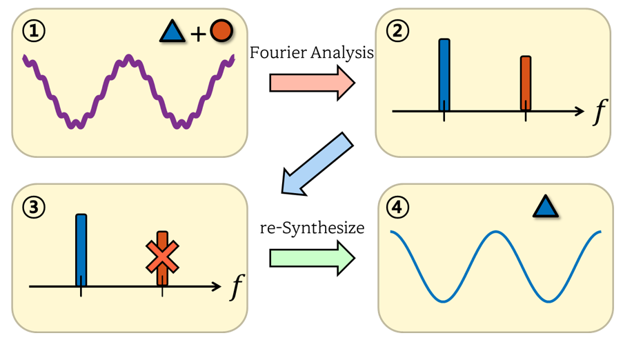
Figure 7. The usefulness of Fourier analysis: it allows for signal analysis on the frequency spectrum and makes it possible to remove unwanted frequency components.

Derivation of Fourier Series

Let’s now mathematically derive the Fourier series, building upon the analogy explained earlier.

Choice of Basis Signals and Spectrum Representation

A vector $(3,4)$ existing on a coordinate plane can be simplified and represented as a linear combination of two different basis vectors, as shown below:

\[(3,4) \Longleftrightarrow 3 \hat{i}+4\hat{j}\]

In a previous post on signal space, we mentioned that a signal can be thought of as a vector.

Similar to how any arbitrary vector can be represented as a linear combination of basis vectors, any arbitrary signal can be represented as a linear combination of basis signals.

For an arbitrary continuous signal $x(t)$ with basis signals $\lbrace \psi_i(t)\rbrace$, it can be represented as a linear combination of basis signals as follows:

\[x(t)=\sum_i c_i \psi_i(t)\]

As you can see, if we know the appropriate set of basis signals $\lbrace \psi_i(t)\rbrace$, we can represent $x(t)$ simply by finding the coefficients $c_i$.

For example, let’s consider an arbitrary continuous signal $x(t)$ and a set of basis signals $\lbrace \psi_i(t)\rbrace$. Suppose that $c_1=1$ and $c_2=3$ for $i=1$, and $c_i=0$ for all other $i$.

Then, it is sufficient to represent this signal by only showing the magnitudes of the basis signals on the $c$ axis.

Like this, the method of representing the original signal using only the magnitudes of the basis signals is called the spectrum representation.

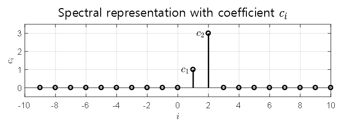
Figure 8. Spectrum representation of an arbitrary continuous signal $x(t)$

---

What characteristics should an appropriate basis signal satisfy in signal processing? Although there are no fixed rules, one reference¹ suggests the following characteristics:

1. It should have a simple shape and be easy to obtain the representation of the signal.
2. It should be able to represent a variety of signals with a wide range of frequencies.
3. The response of the system to the represented signal should be conveniently expressible.
4. There should be only one basic signal corresponding to a single frequency.

And one of the basis functions that best satisfies these four characteristics is the trigonometric function².

However, since trigonometric functions are periodic functions, in order to represent a signal by linear combination of trigonometric functions as a basis signal, the signal to be represented must be a periodic function.

According to Fourier’s result, a periodic signal can be expressed as the sum of a sinusoidal wave with the same period and a sinusoidal wave with a frequency that is an integer multiple of the sinusoidal wave³. Therefore, an arbitrary continuous signal $x(t)$ with period $T$ can be represented as a linear combination of sinusoidal waves as follows:

\[x(t)=a_0+\sum_{k=1}^\infty a_k\cos\left(\frac{2\pi k t}{T}\right)+\sum_{k=1}^{\infty} b_k \sin\left(\frac{2\pi k t}{T}\right)\]

Here, in order to simplify the form of the equation⁴ (condition 1 above) and to conveniently express the system response⁵ (condition 3 above), complex sinusoidal waves rather than real sinusoidal waves are used.

Complex sinusoidals are obtained using Euler’s formula, which is given as follows:

\[\exp(j\theta) = \cos(\theta) + j \sin(\theta)\]

where $j=\sqrt{-1}$

Therefore,

\[\cos(\theta) = \frac{\exp(j\theta)+\exp(-j\theta)}{2}\] \[\sin(\theta) = \frac{\exp(j\theta)-\exp(-j\theta)}{2j}\]

From this, we can rewrite $x(t)$ as follows.

\[x(t)=a_0+\sum_{k=1}^\infty a_k\cos\left(\frac{2\pi k t}{T}\right)+\sum_{k=1}^{\infty} b_k \sin\left(\frac{2\pi k t}{T}\right)\] \[=a_0+\sum_{k=1}^{\infty}\left( a_k\frac{\exp\left(j 2\pi k t/T\right)+\exp\left(-j2\pi k t/T\right)}{2} + b_k\frac{\exp\left(j 2\pi k t/T\right)-\exp\left(-j 2\pi k t/T\right)}{2j} \right)\] \[=a_0+\sum_{k=1}^{\infty}\left( \frac{a_k-jb_k}{2}\exp\left(j\frac{2\pi k t}{T}\right)+\frac{a_k+jb_k}{2}\exp\left(-j\frac{2\pi kt}{T}\right) \right)\] \[=\sum_{k=-\infty}^{\infty}c_k\exp\left(j\frac{2\pi k t}{T}\right)\]

Here, it can be seen that $c_k$ has a relationship with $a_0, a_k, b_k$ as follows.

\[c_k = \begin{cases}\frac{1}{2}(a_k-jb_k),&& k >0 \\ a_0, && k = 0\\ \frac{1}{2}(a_k+jb_k), && k < 0 \end{cases}\]

In conclusion, we can represent any continuous signal $x(t)$ using complex trigonometric functions.

Orthogonality of Complex Sinusoids

One of the reasons why trigonometric functions are useful as basis signals is their orthogonality, which makes it easy to obtain the representation of signals.

Orthogonality between signals means that the inner product between signals is 0. For any arbitrary signals $x(t)$ and $z(t)$ defined over an interval $(a, b)$, if the following condition holds, the two signals are said to be orthogonal:

\[\langle x(t), z(t) \rangle = \int_{a}^{b}x(t)z^*(t) dt= 0\]

For example, let’s consider the inner product of two complex exponentials defined over the interval $(0, T)$:

\[\langle \exp\left(j\frac{2\pi k t}{T}\right), \exp\left(j\frac{2\pi p t}{T}\right)\rangle\] \[=\int_{0}^{T}\exp\left(j\frac{2\pi k t}{T}\right)\exp\left(-j\frac{2\pi p t}{T}\right)dt\] \[=\int_{0}^{T}\exp\left(j\frac{2\pi (k-p) t}{T}\right)dt\]

If $k=p$, then

\[\Rightarrow \int_{0}^{T}\exp(0)dt = T\]

On the other hand, if $k\neq p$, we can substitute $q=k-p$ to get

\[\Rightarrow \int_{0}^{T}\exp\left(j\frac{2\pi q t}{T}\right)dt\] \[= \frac{T}{j2\pi q}\left|\exp\left(j\frac{2\pi q t}{T}\right)\right|_{0}^{T}=\frac{T}{j2\pi q}(\exp(j2\pi q) - \exp(0)) = \frac{T}{j2\pi q}(1-1) = 0\]

Therefore, we can conclude that complex exponentials with different frequencies are orthogonal to each other, and complex exponentials with the same frequency result in an inner product of $T$.

Calculation of Coefficients $c_k$

From equation (10), we can see that

\[x(t)=\sum_{k=-\infty}^{\infty }c_k \exp\left(j\frac{2\pi k t}{T}\right)\]

Now, to calculate $c_k$, we can take the following inner product:

\[\lt x(t), \exp\left(j\frac{2\pi p t}{T}\right)\gt\] \[=\int_{0}^{T}x(t)\exp\left(-j\frac{2\pi p t}{T}\right)dt\] \[=\int_{0}^{T}\sum_{k=-\infty}^{\infty}c_k\exp\left(j\frac{2\pi kt}{T}\right)\exp\left(-j\frac{2\pi pt}{T}\right)dt\] \[=\int_{0}^{T}\sum_{k=-\infty}^{\infty}c_k\exp\left(j\frac{2\pi (k-p)t}{T}\right)dt\]

Considering the results from equations (16) and (18), we have

\[\Rightarrow c_k T\]

Therefore, the coefficients $c_k$ can be calculated as follows:

\[c_k =\frac{1}{T}\int_{0}^{T}x(t)\exp\left(-j\frac{2\pi k t}{T}\right)dt\]

Summary

The Fourier series can be summarized with the following two equations:

For a continuous signal $x(t)$ defined on the interval $(0, T)$ with period $T$,

\[x(t)=\sum_{k=-\infty}^{\infty}c_k\exp\left(j \frac{2\pi k t}{T}\right)\] \[c_k = \frac{1}{T}\int_{0}^{T}x(t)\exp\left(-j\frac{2\pi k t}{T}\right)dt\]

Example

Problem 1. Calculate the Fourier series of the following square pulse.

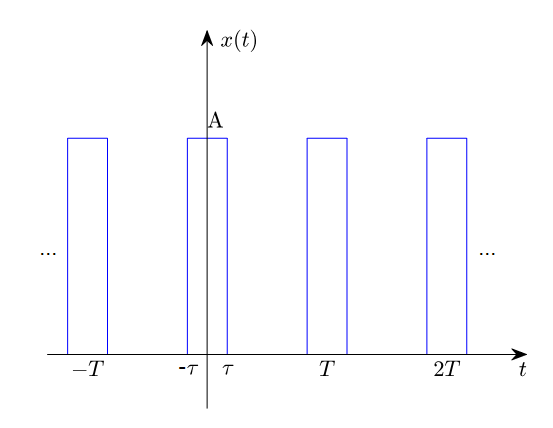
Figure 9. Square pulse periodic signal for Problem 1

From the above figure, it can be observed that the integral can be taken over one period without the function being discontinuous, by choosing the integration interval as $(-T/2, T/2)$.

Therefore, the coefficients $c_k$ of the Fourier series can be calculated as follows:

\[c_k = \frac{1}{T}\int_{-\tau}^{\tau}A\exp\left(-j\frac{2\pi k t}{T}\right)dt=\frac{A}{T}\left(-\frac{T}{j2\pi k}\right)\left|\exp\left(-j\frac{2\pi k t}{T}\right)\right|_{-\tau}^{\tau}\] \[=\frac{A}{T}\frac{T}{(-j2\pi k)}\left\lbrace\cos\left(\frac{2\pi k\tau}{T}\right)-j\sin\left(\frac{2\pi k\tau}{T}\right)-\cos\left(\frac{2\pi k\tau}{T}\right)-j\sin\left(\frac{2\pi k\tau}{T}\right)\right\rbrace\]

\(=\frac{A}{T}\frac{T}{2\pi k}2\sin\left(\frac{2\pi k \tau}{T}\right)\) Here, to match the sine function with the sinc function, we multiply $\tau$ to the numerator and denominator of the second fraction as follows:

\[=\frac{A}{T}\frac{T\tau}{2\pi k\tau}2\sin\left(\frac{2\pi k \tau}{T}\right)\] \[=\frac{2A\tau}{T}\text{sinc}\left(\frac{2k\tau}{T}\right)\]

where the sinc function is defined as follows:

\[\text{sinc}(x)=\frac{\sin(\pi x)}{\pi x}\]

The shape of the sinc function is shown in the following figure:

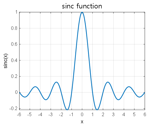
Figure 10. Fourier coefficients (spectrum) of square pulse periodic signal for $T = 3, \tau = 0.5, A = 2$

Now that we have obtained the coefficients, we can express the original signal $x(t)$ as follows:

\[x(t) = \sum_{k=-\infty}^{\infty}c_k\exp\left(j\frac{2\pi k t}{T}\right)=\frac{2A\tau}{T}\sum_{k=-\infty}^{\infty}\text{sinc}\left(\frac{2k\tau}{T}\right)\exp\left(j\frac{2\pi k t}{T}\right)\]

This form represents the series obtained by adding one term at a time from $k=0$ to $k=\pm 1$, $k=\pm 2$, and so on.

Plotting this series using a computer, we can see that it converges to the original square pulse signal shown in Figure 2 as we add more terms with changing $k$.

Figure 11. As the sum of Fourier series terms continues to be added, it becomes similar to the original pulse periodic signal.

On the other hand, when plotting $c_k$ according to changes in $k$, it looks as follows. It retains the shape of the sinc function, with sparse samples visible.

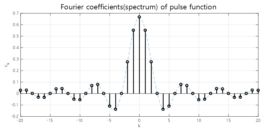
Figure 12. Fourier coefficients (spectrum) of a square pulse periodic signal, with $T = 3$, $\tau = 0.5$, and $A = 2$.

Reference

• Digital Signal Processing, Cheon-Heui Lee, Hanbit Academy.