※ Wold’s theorem can be thought of as the Discrete Time Random Signal version of the Wiener-Kinchin Theorem.

1. The Power Spectrum Density (PSD) of Discrete Time Random Signals

※ The contents of this article is from Introduction to applied statistical signal analysis, 3e. by Richard Shiavi pp.203 - 205

The biggest problem when considering the Fourier transform of a wide-sense stationary random signal is that the Fourier transform may not exist. In other words, $X(f)$ exists only if the signal’s energy is finite. This means that the following equation must be satisfied:

\[energy = T\sum_{n=-\infty}^{\infty}x(n)^2 \lt \infty\]

Since $x(n)$ is at least wide-sense stationary, the energy of all sample functions diverges to positive infinity (Priestly, 1981)¹. In fact, the average energy also diverges to positive infinity.

\[E\lbrace energy\rbrace = T\sum_{n=-\infty}^{\infty}E \lbrace x(n)^2\rbrace = \infty\]

However, instead of average energy, average power can be a finite quantity and can be used as the basis value for frequency transformation. The average power is defined as follows:

\[E\lbrace power\rbrace = \lim_{N\rightarrow \infty}\sum_{n=-N}^{N}\frac{T E\lbrace x(n)^2\rbrace}{(2N+1)T} = E\lbrace x(n)^2\rbrace \lt \infty\]

Here, to include the frequency variable in the equation, let’s define $x_p(n)$ as follows:

\[x_p(n) = \begin{cases}x(n) && |n|\leq N \\ 0 && |n| \gt N \end{cases}\]

According to Parseval’s theorem, the following equation holds:

\[T\sum_{n=-\infty}^{\infty}x_p(n)^2 = \int_{-1/2T}^{1/2T}X_p(f)X^*_p(f) df\]

Since the sequence of $x_p(n)$ is finite, the summation limits above can be changed from $- \infty$ to $\infty$ to $-N$ to $N$. Therefore, the following equation holds.

\[E\lbrace power\rbrace = \lim_{N\rightarrow \infty}E\left\lbrace \sum_{n=-N}^{N}\frac{T x_p(n)^2}{(2N+1)T}\right\rbrace\] \[= \lim_{N\rightarrow \infty}E\left\lbrace \frac{\int_{-1/2T}^{1/2T}X_p(f)X^*_p(f) df}{(2N+1)T}\right\rbrace\]

\(=\int_{-1/2T}^{1/2T}\lim_{N\rightarrow \infty}E\left\lbrace \frac{X_p(f)X^*_p(f)}{(2N+1)T}\right\rbrace df\) Here, the antiderivative function is referred to as power spectral density (PSD).

\[S(f) = \lim_{N\rightarrow \infty} E\left\lbrace \frac{X_p(f) X^*_p(f)}{(2N+1)T}\right\rbrace\]

2. Proof of Wold’s Theorem

The result of Wold’s theorem is as follows.

\[S(f) = T\sum_{k=-\infty}^{\infty}R(k) \exp(-j2\pi fkT)\]

Using the definition of $S(f)$ in equation (9) above, let’s prove this.

Let’s examine the value within the limit in equation (9) more closely.

By the definition of DTFT, the following holds.

\[E\left\lbrace \frac{X_p(f)X^*_p(f)}{(2N+1)T}\right\rbrace = E\left\lbrace \frac{1}{(2N+1)T}\left(T\sum_{n=-N}^{N}x(n)\exp(-j 2\pi fnT)\right)\left(T\sum_{l=-N}^{N}x(l)\exp(-j 2\pi flT)\right)^*\right\rbrace\]

Then, by rearranging the linear operators, we have the following.

\[\Rightarrow \frac{T^2}{(2N+1)T}\sum_{n=-N}^{N}\sum_{l=-N}^{N} E\lbrace x(n)x(l)\rbrace \exp(-j2\pi f(n-l) T)\]

Assuming that the discrete-time signal $x(n)$ is wide-sense stationary, we have the following.

\[\Rightarrow \frac{T}{(2N+1)}\sum_{n=-N}^{N}\sum_{l=-N}^{N}R(n-l)\exp(-j2\pi f(n-l) T)\]

Here, $R(\cdot)$ is the autocorrelation function.

Now, let’s consider how to calculate

\[\sum_{n=-N}^{N}\sum_{l=-N}^{N}R(n-l)\exp(-j2\pi f(n-l) T)\]

We can think of $n$ and $l$ as independent variables. In this case, $n$ and $l$ have the following range.

\[-N\leq n \leq N\] \[-N \leq l \leq N\]

Furthermore, both $n$ and $l$ are discrete variables with an interval of 1.

Therefore, we can consider equation (14) as shown in the figure below. In this case, each point corresponds to the value of $R(n-l) \exp(-j2\pi f(n-l)T)$ for the given values of $n$ and $l$.

That is, although not all black circles are shown in the figure below, all black circles within $-N \leq n \leq N$, $-N \leq n \leq N$ will be completely filled.

Then, we can obtain the same result as equation (14) by summing the values of $R(n-l) \exp(-j2\pi f(n-l)T)$ for each black circle.

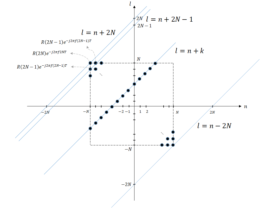
Figure 1.

If we let $k=n-l$, then $l=n-k$, which becomes a first-degree function with a slope of 1. As shown in the figure, we can see that the range of $k$ is $-2N \lt k \lt 2N$.

We can check the values of $R(n-l)\exp(-j2\pi f(n-l)T)$ that need to be added during the transformation of $k$ from $-2N$ to $2N$ as shown below.

\[k=2N \Rightarrow R(2N)\exp(-j2\pi f (2N) T)\] \[k=2N-1 \Rightarrow 2\times R(2N-1)\exp(-j2\pi f (2N-1) T)\] \[k=2N-2 \Rightarrow 3\times R(2N-2)\exp(-j2\pi f (2N-2) T)\] \[\vdots\notag\] \[k=0 \Rightarrow (2N+1)\times R(0)\exp(-j2\pi f (0) T)\] \[\vdots\notag\] \[k=-(2N-2) \Rightarrow 3\times R(2N-2)\exp(-j2\pi f (2N-2) T)\] \[k=-(2N-1) \Rightarrow 2\times R(2N-1)\exp(-j2\pi f (2N-1) T)\] \[k=-2N \Rightarrow R(2N)\exp(-j2\pi f (2N) T)\]

Therefore, for all $k$, the value of equation (14) can be expressed as follows:

\[\sum_{k=-2N}^{2N}(2N+1-|k|)R(k)\exp(-j2\pi fkT)\]

Therefore, the equation (13) that we want to find can be expressed as follows:

\[Equation(13)\Rightarrow \frac{T}{(2N+1)}\sum_{k=-2N}^{2N}(2N+1-|k|)R(k)\exp(-j2\pi fkT)\] \[=T\sum_{k=-2N}^{2N}\left(1-\frac{|k|}{2N+1}\right)R(k)\exp(-j2\pi fkT)\]

Therefore,

\[S(f) = \lim_{N\rightarrow \infty}\sum_{k=-2N}^{2N}T\left(1-\frac{|k|}{2N+1}\right)R(k)\exp(-j2\pi fkT)\] \[=T\sum_{k=-\infty}^{\infty}R(k)\exp(-j2\pi fkT)\]

Also, according to the definition of the DTFT,

\[R(k) =\int_{-1/2T}^{1/2T}S(f)\exp(j2\pi fkT)df\]