이 문서의 한국어 버전은 아래의 위치에서 찾을 수 있습니다. (You can find a Korean version of this article as below.)
Prerequisites
To understand this post well, it is recommended to have knowledge of the following topics:
Unit impulse function
In this post, we will mainly focus on discrete convolution. However, before considering discrete convolution, let’s think about a simple but very important function.
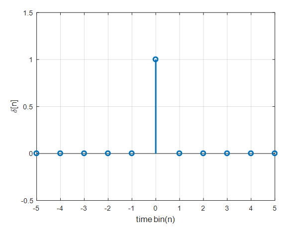
Figure 1. Unit impulse function
The function defined as shown in the above figure is called a unit impulse function. The definition of the unit impulse function is as follows:
\[\delta[n]=\begin{cases}1, &\text{if } n=0 \\ 0, & \text{otherwise}\end{cases}\]The unit impulse function plays the same role as 1 in numbers, and in the case of vectors, it plays the role of a unit basis vector.
Discrete Convolution
Derivation of Discrete Convolution
The unit impulse can be shifted left or right in discrete time. For example, $\delta[n-2]$ is the unit impulse shifted to the right by 2 from $\delta[n]$.
By extending this concept further, we can use the impulse to decompose and represent arbitrary signals. Consider the arbitrary discrete signal $x[n]$ below.
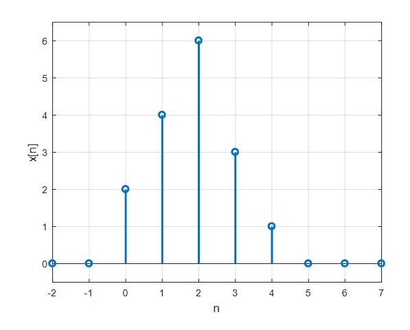
Figure 2. Arbitrary discrete signal $x[n]$
This discrete signal can be expressed as follows using the unit impulse and functions shifted to the left and right of it.
\[x[n]=\sum_{k=-\infty}^{\infty}x[k]\delta[n-k]\] \[=\cdots + x[-2]\delta[n+2]+x[-1]\delta[n+1]+x[0]\delta[n]+x[1]\delta[n-1]+x[2]\delta[n-2]+\cdots\]In other words, an arbitrary function $x[n]$ can be decomposed using the function $\delta [n-k]$.
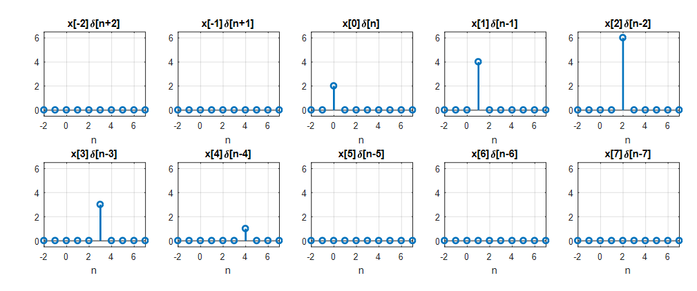
Figure 3. Result of decomposing an arbitrary discrete function $x[n]$ using unit impulse functions
Equation (3) can be seen as decomposing $x[n]$ using unit impulse functions or as a sum of a sequence of signals multiplied by constants.
Here, the constant refers to $x[k]$, which represents the $k$-th function value and is no longer a function but a constant.
Equation (3) is also written as follows.
\[\Rightarrow x[n] * \delta[n]\]The operation $*$ is also called convolution.
In general, the convolution of two arbitrary discrete functions $x[n]$ and $h[n]$ is as follows.
\[x[n] * h[n] = \sum_{k=-\infty}^{\infty}x[k]h[n-k]\]LTI Systems and Convolution
Let’s think of the relationship between input $x[n]$ and output $y[n]$ as a transformation of $x[n]$ to $y[n]$, denoted as $y[n]=T\left(x[n] \right)$.
If the system being considered is an LTI system, then by linearity, the following holds:
\[T\left( \sum_{k=-\infty}^{\infty}c_kx_k[n]\right) = \sum_{k=-\infty}^{\infty}{c_kT(x_k[n])}=\sum_{k=-\infty}^{\infty}{c_ky_k[n]}\]Furthermore, by time-invariance, the following holds:
\[T \left(x[n-k] \right)=y[n-k]\]Using Equation (3) again, let’s expand the following equation:
\[y[n] =T(x[n])\notag\] \[=T\left(\cdots + x[-2]\delta[n+2]+x[-1]\delta[n+1]+x[0]\delta[n]+x[1]\delta[n-1]+x[2]\delta[n-2]+\cdots \right)\] \[=T\left( \sum_{k=-\infty}^{\infty}{x[k]\delta[n-k]}\right)\]Since $x[k]$ is a constant with respect to $n$, we can use linearity to rewrite the above equation as:
\[\Rightarrow \sum_{k=-\infty}^{\infty}{\left(x[k]T\left(\delta[n-k]\right) \right)}\]Let’s define $h[n]=T\left(\delta[n]\right)$, then by time-invariance,
\[\Rightarrow \sum_{k=-\infty}^{\infty}{\left(x[k]T\left(\delta[n-k]\right) \right)} = \sum_{k=-\infty}^{\infty}{x[k]h[n-k]}\]Therefore,
\[y[n] = \sum_{k=-\infty}^{\infty}{x[k]h[n-k]}\]Here, $h[n] = T\left(\delta[n]\right)$ is the response of the system when the input is an impulse, which is called the impulse response.
In other words, if the system being considered is an LTI system, then the input-output relationship of the system can be expressed as the discrete convolution between the input and impulse response of the system.
Discrete Convolution Properties
Commutative Property
Convolution satisfies the commutative property, which means that for two signals $x[n]$ and $h[n]$, the following equation holds:
\[x[n] * h[n] = h[n] * x[n]\]By examining the definition of convolution in equation (5), we can see that one of the signals is flipped and added. The commutative property implies that the order of the two signals does not affect the result. Therefore, we can flip the signal that is easier to compute and perform the operation.
From a system perspective, it means that the output of the system remains the same even if we swap the roles of the input signal and the impulse response.
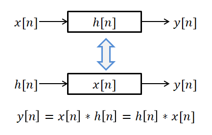
Figure 4. The commutative property of discrete convolution implies that the system output remains the same even if the input signal and the impulse response roles are exchanged.
Alternatively, we can interpret the commutative property to mean that when two systems are connected in series, the order of the systems can be reversed without affecting the overall system.
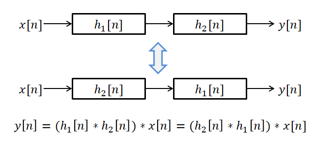
Figure 5. The commutative property of discrete convolution implies that the order of the systems applied in series can be reversed without affecting the overall system.
Associative Property
Convolution satisfies the associative property, which means that the order of the calculation of the combined convolution of three or more signals does not depend on the order in which they are grouped.
\[(x[n] * h_1[n]) * h_2[n] = x[n] * (h_1[n] * h_2[n])\]For example, when two systems are connected in series, we can use one system that combines both systems’ impulse responses to replace the convolution of the two systems.
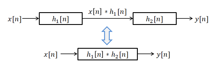
Figure 6. The associative property of discrete convolution. We can treat the two systems as one system by combining their impulse responses with convolution.
Distributive Property
Convolution satisfies the distributive property over addition, which means that the convolution operation distributes over addition.
\[x[n]*(h_1[n] + h_2[n])= x[n]*h_1[n] + x[n]*h_2[n]\]The distributive property implies that if two systems are connected in parallel, the overall system can be replaced by the sum of their impulse responses.
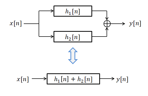
Figure 7. The distributive property of discrete convolution. We can replace the parallel connection of two systems by the sum of their impulse responses with convolution.
Impulse response
Physical meaning of impulse response
Impulse response is the output of a system when an impulse is given as an input, which is obtained as a result of inducing discrete convolution.
However, the impulse response has a greater significance than this. The impulse response serves as a weight that reveals how much the past input values contribute to the current output value.
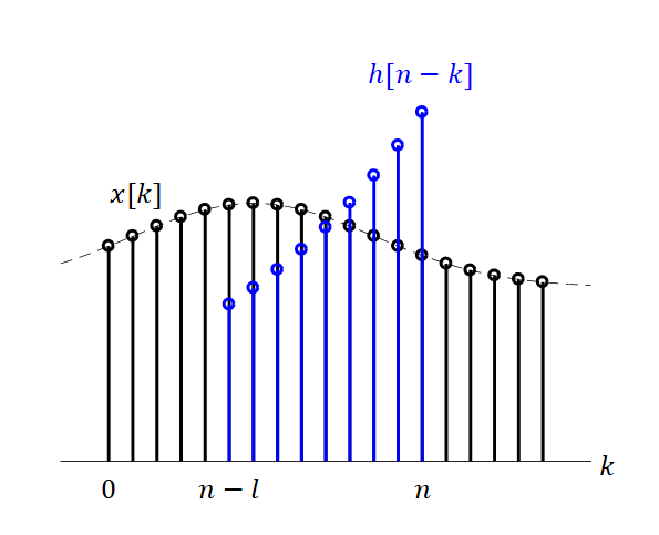
Figure 8. Physical meaning of impulse response
Therefore, it is possible to understand the characteristics of a system by having only its impulse response.
Also, supplying an impulse input can be considered as giving a kind of start to the system. By giving an impulse input at $n=0$, the system operates at $n>0$, which reflects the internal characteristics of the system rather than a response to external input. Hence, information about the characteristics of the system can be obtained through the impulse response.
Impulse response and system characteristics
In the previous post on Linear Time-Invariant (LTI) systems, we learned about linear and time-invariant systems, but there are also other characteristics of systems that can be considered.
Instantaneous systems and dynamic systems
An instantaneous system refers to a system that is determined only by the current input. In contrast, a dynamic system can be influenced by past outputs or inputs.
An example of an instantaneous system is as follows:
\[y[n]=3x[n]\]Here, the impulse response would be $h[n]=3$.
On the other hand, an example of a dynamic system is as follows:
\[y[n]=\frac{1}{2}(x[n]+x[n-1])\]In this case, the impulse response is as follows (the reason why will be explained in the following problem):
\(h[n]=\frac{1}{2}(\delta[n]+\delta[n-1])=\begin{cases} 0.5 & n = 0, 1 \\ 0 & \text{otherwise} \end{cases}\)
Causal and Non-causal Systems
Causal systems are systems that require input in order to produce an output. In other words, the output is zero until an input is provided. These are systems for which $h[k]=0$ when $k<0$.
One characteristic of a causal system is that it only uses past inputs. To understand this, we can use convolution to rewrite the input-output relationship as follows:
\[y[n]=\sum_{k=-\infty}^{\infty}h[k]x[n-k]\] \[=\sum_{k=-\infty}^{-1}h[k]x[n-k]+\sum_{k=0}^{\infty}h[k]x[n-k]\]Looking at the second equation above, we can see that the first term uses $x[n+1]$ and $x[n+2]$, while the second term uses $x[n]$ and $x[n-1]$, and so on. Therefore, if a system is causal, it only uses past inputs such as $x[n]$ and $x[n-1]$, and if $h[n]=0$ for $n<0$, the system only uses past inputs to compute the current output.
Stable and Unstable Systems
The conditions for a system to be stable or unstable are that the input and output magnitudes must be finite.
In practice, it is not possible to create a system that diverges infinitely because the output voltage or numerical value that can be output is limited. However, theoretically, a system that has an output that diverges to infinity is called an unstable system.
This is also referred to as “Bounded Input Bounded Output” or BIBO stability.
If the input $x[n]$ is bounded by a finite value such that
\[|x[n]|\lt B_x\]Then, for the output to also have a finite magnitude, we must satisfy the following condition:
\[|y[n]|=\left|\sum_{k=-\infty}^{\infty}h[k]x[n-k]\right|\leq\sum_{k=-\infty}^{\infty}|h[k]||x[n-k]|\] \[\leq B_x\sum_{k=-\infty}^{\infty}|h[k]|\]Therefore, for a system to be BIBO stable, the impulse response must be absolutely summable, which means it satisfies the following condition:
\[\sum_{k=-\infty}^{\infty}|h[k]|<\infty\]Classification of Finite/Infinite Impulse Response based on the length of impulse response
Depending on whether the length of the impulse response is finite or infinite, the systems are distinguished as Finite Impulse Response (FIR) and Infinite Impulse Response (IIR) systems.
In fact, the distinction between FIR and IIR systems plays a very important role even when designing filters.
For example, the following system is an FIR system.
\[y[n]=ax[n]+bx[n-1]\]In this case, the impulse response is
\[h[n]=a\delta[n]+b\delta[n-1]\]On the other hand, the following system is an IIR system.
\[y[n]+ay[n-1]=bx[n]\]In this case, the impulse response is as follows.
\[h[n]=(-a)^nb\text{,}\ \ \ n\geq 0\]Example
Problem 1.
For the moving average system with the input-output relationship as follows:
\[y[n]=\frac{1}{2}\left(x[n]+x[n-1]\right)\]1) Determine whether this system is an LTI system.
First, let’s determine if the system is linear.
Let’s name the system as $\mathcal{T}(\cdot)$.
If the following equation holds, then the system is linear:
\[\mathcal{T}(\alpha x_1[n]+\beta x_2[n])=\alpha\mathcal{T}(x_1[n])+\beta\mathcal{T}(x_2[n])\]The left-hand side is as follows:
\[\mathcal{T}(\alpha x_1[n]+\beta x_2[n])=\frac{1}{2}\left\lbrace\alpha x_1[n]+\beta x_2[n] +\alpha x_1[n-1] + \beta x_2[n-1]\right\rbrace\]The right-hand side is as follows:
\[\alpha\mathcal{T}(x_1[n])+\beta\mathcal{T}(x_2[n]) = \alpha \left(\frac{1}{2}(x_1[n]+x_1[n-1]\right)+\beta \left(\frac{1}{2}(x_2[n]+x_2[n-1]\right)\]Therefore, since the left and right-hand sides are the same, the system is linear.
Now let’s check if the system is time-invariant. If the following equation holds, then the system is time-invariant:
\[\mathcal{T}(x[n-k]) = y[n-k]\]The left-hand side is as follows:
\[\mathcal{T}(x[n-k]) = \frac{1}{2}\left(x[n-k]+x[n-k-1]\right)\]The right-hand side is as follows, and it is the same as the left-hand side:
\[y[n-k]=\frac{1}{2}\left(x[n-k]+x[n-k-1]\right)\]Therefore, the system is both linear and time-invariant.
In summary, this system is a linear time-invariant system.
2) Calculate the impulse response of this system.
The impulse response $h[n]$ is the response when the input is $x[n]=\delta[n]$. Therefore, the impulse response is as follows:
\[h[n]=\frac{1}{2}(\delta[n]+\delta[n-1])=\begin{cases} 0.5 & n = 0, 1 \\ 0 & \text{otherwise} \end{cases}\]3) Calculate the output for a specific input.
Given the input as follows, calculate the output:
\[x[n]=\begin{cases} 1 & n = 0, 1, 2 \\ 0 & \text{otherwise} \end{cases}\]In an LTI system, the input-output relationship can be calculated as the convolution of the input and impulse response.
Therefore, the output value is as follows:
\[y[n]=h[n] * x[n]\] \[=\sum_{k=-\infty}^\infty h[n-k]x[k]\]Therefore, considering all possible values of n, $y[n]$ is as follows:
When $n=-1$, $y[-1]=\cdots + x[-1]h[0]+x[0]h[-1]+x[1]h[-2]+x[2]h[-3]+\cdots = 0$
When $n=0$, $y[0]=\cdots + x[-1]h[1]+x[0]h[0]+x[1]h[-1]+x[2]h[-2]+\cdots = 0.5$
When $n=1$, $y[1]=\cdots + x[-1]h[2]+x[0]h[1]+x[1]h[0]+x[2]h[-1]+\cdots = 1$
When $n=2$, $y[2]=\cdots + x[-1]h[3]+x[0]h[2]+x[1]h[1]+x[2]h[0]+\cdots = 1$
When $n=3$, $y[3]=\cdots + x[-1]h[4]+x[0]h[3]+x[1]h[2]+x[2]h[1]+\cdots = 0.5$
When $n=4$, $y[4]=\cdots + x[-1]h[5]+x[0]h[4]+x[1]h[3]+x[2]h[2]+\cdots = 0$
The process can be represented in the following graph.
Figure 9. The procedure to calculate output via discrete convolution
Used GUI: Discrete Convolution Demo of DSP First's MATLAB GUI
Problem 2.
For the autoregressive system with the input-output relationship as follows,
\[y[n] = a y[n-1] + b x[n]\]assuming the following conditions:
\[x[n] = 0 \text{ for } n\lt 0\] \[y[n]=0 \text{ for }n=-\infty\]1) Determine whether this system is an LTI system.
To determine whether this system is an LTI system, we need to modify the input-output relationship of the system.
Due to the condition that $y[-\infty]=0$, we have $y[-1]=0$ when $n=-1$.
Also, when $n=0$, $y[0]=b x[0]$. Similarly, for $n=1,2,\cdots$,
\[y[1]=ab x[0]+b x[1]\] \[y[2] = a^2b x[0]+ab x[1] + b x[2]\] \[\vdots \notag\] \[y[n]=\sum_{k=0}^{n}a^k b x[n-k]\]Now, let’s use the above equation to determine linearity and time-invariance.
First, let’s determine linearity.
Let’s name the system as $\mathcal{T}(\cdot)$.
If the following holds, the system is linear:
\[\mathcal{T}(\alpha x_1[n]+\beta x_2[n])=\alpha\mathcal{T}(x_1[n])+\beta\mathcal{T}(x_2[n])\]The left-hand side is as follows: \(\mathcal{T}(\alpha x_1[n]+\beta x_2[n])=\alpha\left[\sum_{k=0}^{n}a^k b x_1[n-k]\right]+\beta\left[\sum_{k=0}^{n}a^k b x_2[n-k]\right]\) The right-hand side of the equation is as follows:
\[\alpha\mathcal{T}(x_1[n])+\beta\mathcal{T}(x_2[n]) = \sum_{k=0}^{n}a^k b\left[\alpha x_1[n-k]+\beta x_2[n-k]\right]\]Therefore, since the left-hand side and the right-hand side are equal, this system is a linear system.
Now let’s determine time-invariance. If the following holds, the system is time-invariant:
\[\mathcal{T}(x[n-\tau]) = y[n-\tau]\]Here, the left-hand side is as follows:
\[\mathcal{T}(x[n-\tau]) = \sum_{k=0}^{n}a^k b x[n-\tau-k]\]However, the values from $n-\tau+1$ to $n$ within the summation notation are equal to 0.
This is because each $x[k]$ value corresponds to $x[-\tau]$ from $x[n-\tau-(n-\tau+1)] = x[-1]$ to $x[n-\tau-n]=x[-\tau]$, and $x[k]=0 \text{ for } k<0$.
Therefore, the left-hand side expression can be rewritten as follows:
\[\Rightarrow \sum_{k=0}^{n-\tau}a^k b x[n-\tau-k]\]Also, the right-hand side is as follows, which is the same as the left-hand side:
\[y[n-\tau]=\sum_{k=0}^{n-\tau}a^k b x[n-\tau-k]\]Therefore, this system is also a time-invariant system.
In summary, this system is a linear time-invariant system.
2) Find the impulse response of this system.
Based on the input-output relationship created to determine the LTI property above,
\[y[n]=\sum_{k=0}^{n}a^k b x[n-k]\]and the impulse response is
\[h[n]=a^n b\]3) Calculate the output for a specific input.
Calculate the output for the following input:
\[x[n]=\begin{cases} 1 & n = 0, 1, 2 \\ 0 & \text{otherwise} \end{cases}\]In an LTI system, the input-output relationship can be calculated as the convolution of the input and the impulse response.
When $n=0$, $y[0]=a^0 b x[0] = b$
When $n=1$, $y[1]=\sum_{k=0}^{1}a^k b x[1-k] = a^0 b x[1-0] + a^1 b x[1-1] = b + ab$
When $n=2$, $y[2]=\sum_{k=0}^{2}a^k b x[2-k] = a^0 b x[2-0] + a^1 b x[2-1] + a^2 b x[2-2] = b + ab+a^2b$
Using this method, we can see that
\[y[n] = a^{(n-2)}b + a^{(n-1)}b+a^n b\]In the figure below, the case where $a=0.8$ and $b=1$ is considered, and the impulse response is shown for only the first 10 samples.
Figure 10. The process of calculating the output value through discrete convolution
Used GUI: Discrete Convolution Demo in DSP First's MATLAB GUI
Reference
- “Signal Processing First”, James H. McClellan et al., Prentice Hall
- “Digital Signal Processing”, Chul Hee Lee, Hanbit Media