Formula of Stokes’ theorem

The formula of Stokes’ theorem can be written as follows:

\[\oint_c\vec{F}\cdot d\vec{r} = \iint_S(\vec{\nabla}\times\vec{F})\cdot d\vec{S}\]

Looking at equation (1), we can see that it is very similar to the formula for Green’s theorem. The formula for Green’s theorem is as follows:

\[\oint_c\vec{F}\cdot d\vec{r} = \iint_A(\vec{\nabla}\times\vec{F})_{2D} dA\]

Here, $(\vec{\nabla}\times\vec{F})_{2D}$ means 2D curl, and the formula is the same as the curl formula, but we use only the magnitude of the curl because there is no longer a vector to represent the $\hat k$ direction in two dimensions.

Comparing equation (1) and equation (2), we can say that Green’s theorem explains the relationship between line integrals and double integrals, while Stokes’ theorem explains the relationship between line integrals and surface integrals.

Stokes’ theorem can be thought of as the three-dimensional version of Green’s theorem. The generalized Stokes’ theorem can deal with more high-dimensional manifolds, but we will focus on understanding and proving it at the level of three dimensions that we need.

The Meaning of Stokes’ Theorem

prerequisites

To understand the meaning of Stokes’ theorem, it is recommended to know the following topics:

• Green’s theorem
• Line integrals of vector fields
• Surface integrals of vector fields
• Rotation of vector fields

In particular, we highly recommend understanding Intuitive understanding of Green’s theorem through Curl.

Introduction to the Meaning of Stokes’ Theorem

Suppose we have a surface S with an enclosed curve C on a vector field as shown below in three-dimensional space.

Figure 1. Let's assume an arbitrary surface S and enclosed curve C on the 3D space.

Assuming that there is a vector field $\vec{F}$ in this 3-dimensional space, the following equation holds by the Stokes’ theorem:

\[\oint_C\vec{F}\cdot d\vec{r} = \iint_S(\vec{\nabla}\times\vec{F})\cdot d \vec{S}\]

The left-hand side of equation (3) is the line integral of the vector field along the curve C.

Now let’s derive the right-hand side of equation (3) from the left-hand side. Let’s split the surface S in half as shown below.

Figure 2. Surface S expressed as two curves.

Looking at Figure 2 from above, we have:

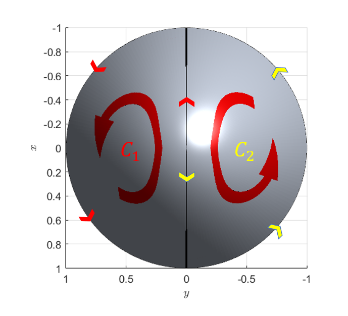
Figure 3. Line integral paths when surface S is divided into two closed curves.

As shown in Figure 3, we call the closed paths that are split into two $C_1$ and $C_2$, respectively.

Also, if we consider the line integral paths of $C_1$ and $C_2$, the length of the line integral path is the same in the middle section, but the direction is opposite, so the values of the line integral cancel out in this region.

Therefore, we can think of the following relationship:

\[\oint_C\vec{F}\cdot d\vec{r} = \oint_{C_1}\vec{F}\cdot d\vec{r} + \oint_{C_2}\vec{F}\cdot d\vec{r}\]

Now let’s try to divide the surface S into four equal parts as shown below.

Figure 4. Surface S expressed as four curves.

Looking at Figure 4 from above, we have:

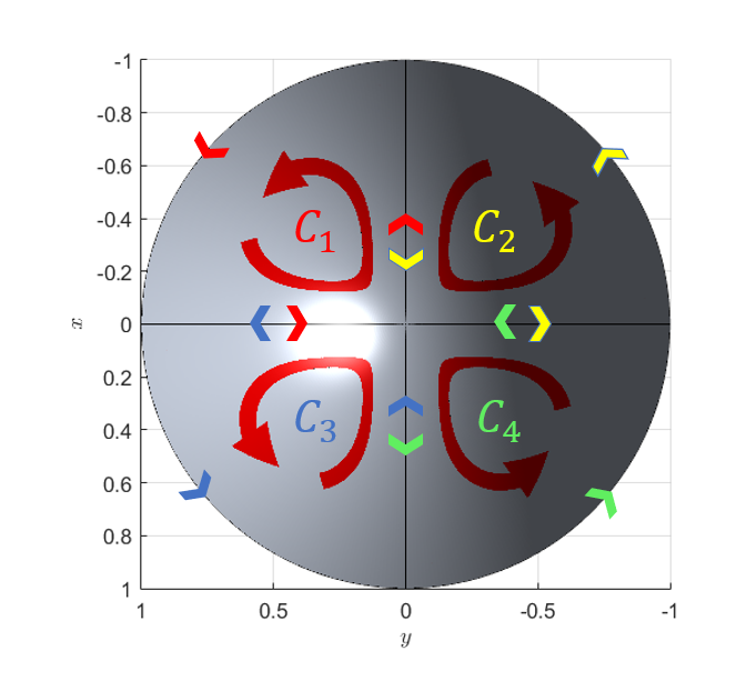
Figure 5. Path of line integrals when dividing the surface S into two closed curves.

By the same logic as before, when dividing the surface into two, the length of the line integral within the path remains the same, but the direction is reversed. Therefore, by summing the line integrals of the four closed paths from $C_1$ to $C_4$ within the path, the value of the line integral for the original outermost path can be obtained.

\[\oint_C\vec{F}\cdot d\vec{r} = \sum_{k=1}^4\oint_{C_k}\vec{F}\cdot d\vec{r}\]

Then, what happens if the surface S is divided into N parts?

Figure 6. Representation of surface S divided into many closed curves.

As with the previous logic, the following equation still holds true no matter how many closed curves are used to divide the surface.

\[\oint_C\vec{F}\cdot d\vec{r} = \sum_{k=1}^N\oint_{C_k}\vec{F}\cdot d\vec{r}\]

Consider the small surface area that is divided into N parts. The line integral within this small path represents the curl of the vector field on the infinitesimal path.

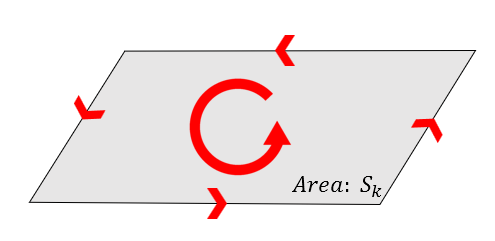
Figure 7. Path and line integral within the small surface area.

As we saw in the section on curl, curl represents the rotational force received by the unit area. Therefore, the rotational amount on a surface area of size $dS$ can be thought of as the product of the curl and the surface area. Additionally, since the direction of the curl vector and the normal vector of the surface are the same, the product of the magnitude of the curl and the surface area is equal to the dot product of the curl vector and the surface normal vector.

Therefore, we can think as follows:

\[\oint_{C_k}\vec{F}\cdot d\vec{r}\approx(\vec\nabla\times\vec F)_{C_k}\cdot \vec{S}_k\]

Thus, rewriting equation (6) gives:

\[Equation(6) = \sum_{k=1}^N\oint_{C_k}\vec{F}\cdot d\vec{r} \approx \sum_{k=1}^N(\vec\nabla\times\vec F)_{C_k}\cdot \vec{S}_k\]

If we make $N$ infinitely large in equation (8), $\vec{S}_k$ will become $d\vec{S}$ and equation (6) will ultimately become:

\[\oint_C\vec{F}\cdot d\vec{r} = \iint_S(\vec{\nabla}\times\vec{F})\cdot d\vec{S}\]

Thus, the Stokes’ theorem holds regardless of the shape of the surface S, as long as the shape of the closed path C is maintained.

Figure 8. Regardless of the shape of the surface S, as long as the shape of the closed path C is maintained, the Stokes' theorem always holds.

Proof of Stokes’ Theorem

prerequisites

To understand the proof process of Stokes’ Theorem well, it is recommended to have knowledge about the following four topics:

• Line Integral of Vector Fields
• Surface Integral of Vector Fields
• Green’s Theorem
• Chain Rule of Partial Differentiation

The necessary chain rules for this context are as follows:

1) for a function $f(x, y, g(x,y))$

\[\frac{\partial}{\partial x}f(x,y,g(x,y)) = \frac{\partial f}{\partial x} + \frac{\partial f}{\partial g}\frac{\partial g}{\partial x}\]

2) for two functions $f(x, y, z)$ and $h(x,y,z)$

\[\frac{\partial}{\partial x}(f\cdot h) = \frac{\partial f}{\partial x}h + f \frac{\partial h}{\partial x}\]

3) for a function $f(x(t), y(t))$

\[\frac{df}{dt}=\frac{\partial f}{\partial x}\frac{dx}{dt} + \frac{\partial f}{\partial y}\frac{dy}{dt}\]

These three chain rules will be used at various points during the proof process, so it is recommended to familiarize yourself with them in advance if there are any difficult parts.

Introduction of the surface and domain for the proof

In this proof process, we will prove Stokes’ Theorem using a function whose domain is the $x$, $y$ plane and whose height is defined as $z=g(x,y)$.

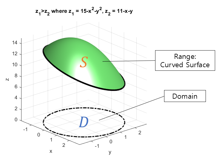
Figure 9. The domain for the proof of Stokes' Theorem is a region with x and y as the domain and height as a function of x and y, along with a closed path (solid black line) and its projection (dotted line).

Afterward, we can prove Stokes’ Theorem for the general 3-dimensional space using a similar method for the case where the domain is $x$, $z$ or $y$, $z$. Here, we denote the given vector field in 3-dimensional space as $\vec{F}$ with $\lt P, Q, R\gt$. The angled brackets represent a shortened form of the original $\vec{F} = P(x,y,z)\hat i +Q(x,y,z)\hat j + R(x,y,z)\hat k$.

Stokes’ Theorem can be expressed in the following equation:

\[\oint_c\vec{F}\cdot d\vec{r} = \iint_S(\vec{\nabla}\times\vec{F})\cdot d\vec{S}\]

Calculation of Surface Integral

Here, let’s start by proving the surface integral part.

\[\iint_S(\vec{\nabla}\times\vec{F})\cdot d\vec{S}\]

Let’s first calculate only the curl part of the vector field.

\[\vec{\nabla}\times\vec{F} = \begin{vmatrix} \hat{i} && \hat{j} && \hat{k} \\ \frac{\partial}{\partial x} && \frac{\partial}{\partial y} && \frac{\partial}{\partial z} \\ P && Q && R \end{vmatrix}\] \[=\lt R_y-Q_z, P_z- R_x, Q_x - P_y \gt\]

Here, the notation $R_y$, etc. can be thought of as the partial derivative of $R$ with respect to $y$.

Also, considering the surface vector $d\vec{S}$, the general equation representing a curved surface using two parameters can be expressed as follows:

\[\vec{r}(u,v) = x(u,v)\hat{i} + y(u,v)\hat{j} + z(u,v)\hat{k}\]

In this case, since the two parameters correspond to $x$ and $y$, the equation of the surface can be expressed as follows:

\[\vec{r}(x,y) = x\hat{i} + y\hat{j} + z\hat{j} = x\hat{i} + y\hat{j} + g(x,y)\hat{k} = \lt x, y, g(x,y)\gt\]

Therefore, as we learned in the surface integral of vector field, the surface vector $d\vec{S}$ is as follows:

\[d\vec{S} = \vec{r}_x\times\vec{r}_y dxdy = \begin{vmatrix}\hat{i} && \hat{j} && \hat{k} \\ 1 && 0 && g_x \\ 0 && 1 && g_y\end{vmatrix}dxdy\] \[=\lt -g_x, -g_y, 1\gt\]

Therefore, equation (14) can be expressed as follows:

\[Equation (14)\Rightarrow \iint_S \lt R_y-Qz, P_z-R_x, Q_x-P_y\gt\cdot\lt -g_x, -g_y, 1\gt dxdy\] \[=\iint_D \left( g_x(Q_z-R_y) + g_y(R_x - P_z) + Q_x-P_y\right) dxdy\]

Since there is nothing else we can do here, let’s move on to the calculation of the line integral part of Stoke’s theorem.

Calculation of line integrals

\[\oint_C\vec{F}\cdot d\vec{r}\]

To calculate the line integral, let’s define the closed path on the original surface as $C$, and the projection of the domain of $C$ onto the surface as $C_0$, as shown in Figure 10 below.

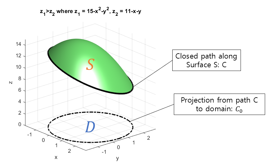
Figure 10. Closed path C and its projection C_0 onto the surface

Then, we can think of the parameter equation for the curve on $C_0$ as follows.

\[\vec{r}_{C_0} = \lt x(t), y(t)\gt\text{ where }a\leq t \leq b\]

Similarly, the parameter equation for the curve on the closed path $C$ can be thought of as follows. Here, $a$ and $b$ are arbitrary real numbers such that $a\lt b$.

\[\vec{r}_C = \lt x(t), y(t), g(x(t), y(t))\gt\text{ where }a\leq t \leq b\]

Now let’s consider the differential displacement $d\vec{r}$ for the closed curve $C$. First, let’s differentiate $r$ with respect to $t$ to compute $d\vec{r}$. Applying the partial differentiation chain rule 3) (Equation (12)) introduced in the early part of the proof of Stokes’ Theorem, we get:

\[\frac{d\vec{r}}{dt} = \lt \frac{dx}{dt}, \frac{dy}{dt}, g_x \frac{dx}{dt} + g_y \frac{dy}{dt}\gt\]

Then, multiplying both sides by $dt$, we have:

\[d\vec{r} = \lt dx, dy, g_x dx + g_y dy\gt\]

Therefore, since $\vec{F}$ is given, $\vec{F}\cdot d\vec{r}$ can be expressed as follows:

\[\vec{F}\cdot d\vec{r} = \lt P, Q, R \gt \cdot \lt dx, dy, g_x dx + g_y dy\gt = Pdx + Qdy + R g_x dx + Rg_y dy\]

Using this, the line integral in Equation (23) can be converted into an integral with respect to $t$:

\[Equation(23)\Rightarrow \int_{t=a}^{t=b}Pdx+Qdy+Rg_xdx+Rg_ydy\]

Grouping $dx$ and $dy$ together, we get:

\[\Rightarrow \int_{t=a}^{t=b}(P+Rg_x)dx + (Q+Rg_y)dy\]

Applying Green’s Theorem, we can convert the line integral on a closed path in a two-dimensional plane into a double integral.

\[\Rightarrow \iint_D(Q+Rg_y)_x - (P+Rg_x)_y dxdy\]

The subscripts $x$ and $y$ behind the parentheses here represent partial derivatives with respect to $x$ and $y$, respectively.

Now, let’s perform the two partial derivative calculations in equation (31) separately.

Calculation of the partial derivative of (Q+Rg_y)_x

Taking the partial derivative of the front part of equation (31), we have:

\[(Q+Rg_y)_x = \frac{\partial}{\partial x}\left( Q(x, y, g(x,y)) + R(x, y, g(x,y))g_y(x, y) \right)\]

Using the first equation (10) and the second equation (11) of the chain rule for partial derivatives, introduced in the beginning of the proof, the above equation can be written as:

\[\Rightarrow Q_x + Q_g g_x + (R_x+R_g g_x)g_y + Rg_{yx}\]

Here, $Q_g$ and $R_g$ can be replaced with $Q_z$ and $R_z$, respectively, as $z=g(x,y)$.

\[\Rightarrow Q_x + Q_z g_x + (R_x+R_z g_x)g_y + Rg_{yx}\]

Calculation of the partial derivative of (P+Rg_x)_y

Taking the partial derivative of the back part of equation (31), we have:

\[(P+Rg_x)_y = \frac{\partial}{\partial y}\left( P(x,y,g(x,y)) + R(x,y,g(x,y))g_x(x,y) \right)\]

Using the first equation (10) and the second equation (11) of the chain rule for partial derivatives, introduced in the beginning of the proof, the above equation can be calculated as:

\[\Rightarrow P_y+P_z g_y + (R_y + R_z g_y)g_x + Rg_{xy}\]

Combining the two partial derivative calculations,

To calculate equation (31), let’s subtract the result of equation (36) from the result of equation (34).

\[Equation(34)-Equation(36) = \left\lbrace Q_x+Q_zg_x+(R_x+R_zg_x)g_y +Rg_{yx}\right\rbrace \notag\] \[- \left\lbrace P_y+P_zg_y + (R_y+R_zg_y)g_x + Rg_{xy}\right\rbrace\] \[=Q_x-P_y + Q_xg_x-P_zg_y+R_xg_y-R_yg_x\] \[=g_x(Q_z-R_y) + g_y(R_x-P_z) + Q_x-P_y\]

Therefore, equation (31) can be written as:

\[Equation(31) = \iint_D \left\lbrace g_x(Q_z-R_y) + g_y(R_x-P_z) + Q_x-P_y\right\rbrace dxdy\]

Verification of the Consistency between the Result of the Surface Integral and that of the Line Integral

So far, we have performed calculations from both the surface integral and the line integral to prove the Stokes’ theorem. If we examine the final results of each calculation, we can see that equation (22) and equation (40) are identical.

The Stokes’ Theorem in a General Three-dimensional Space

Previously, we proved the Stokes’ theorem for the case of a surface $S: g(x,y)$, where $S$ is a function of $x$ and $y$. Using the same method, we can also prove the theorem for surfaces with $S: g(x,z)$ or $S: g(y,z)$, so we can conclude that the Stokes’ theorem holds in a general three-dimensional space with any type of surface.