In this post, we aim to derive the formula for the normal distribution (or Gaussian distribution).
Since the formula for the normal distribution is quite complicated, we will break it down into three parts, as shown in the figure below.
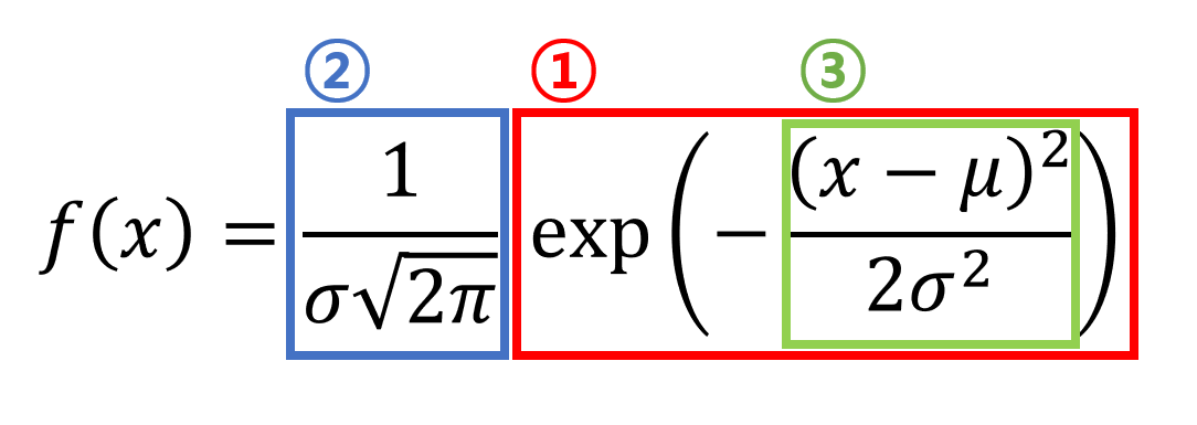
Figure 1. Formula for the normal distribution and derivation order in the post
Prerequisites
To understand this post, it is recommended that you have a good understanding of the following:
- Concept and characteristics of probability density function
- Gaussian integral
Derivation of the form $e^{-x^2}$
First, let’s derive the fact that $f(x)$ follows the form of $e^{-x^2}$.
Necessary assumptions
To do this, let’s imagine throwing darts onto a circular dartboard with the center aligned with the origin of a Cartesian coordinate system, as shown below.
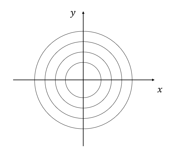
Figure 2. Circular dartboard with center aligned at the origin
Necessary assumptions:
- If we represent the score on the dartboard with contour lines, then darts that hit the same contour line have the same score. In other words, the probability density function is independent of rotation.
- Assuming we throw darts that hit within a square target, if the area of the square target is the same, then the closer the distance from the origin to the square, the higher the probability of hitting the target.
- When the distance from the origin to the square is the same, the larger the area of the square, the higher the probability of hitting the target.
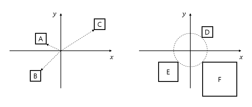
Figure 3. (Left) If the size of the squares is the same, the probability of hitting the square is higher when the distance is closer. In other words, the order of the squares with the highest probability of hitting is A, B, and C. (Right) When the distance to the square is the same, the probability of hitting the square is higher as the area of the square is wider. In other words, the order of the squares with the highest probability of hitting is F, E, and D.
Derivation Process
Let’s consider the expected value of hitting a square $A$ with width $\Delta x$ and height $\Delta y$ at an arbitrary position $(x,y)$ on the orthogonal coordinate system, while thinking about the three assumptions mentioned earlier.
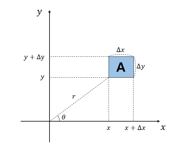
Figure 4. Square A to calculate the expected value.
Let $f(x,y)$ be the probability density function for a dart to land on the $x$ and $y$ axes. Since the probability of a dart landing on the $x$ and $y$ axes are independent, the probability density functions for a dart landing on the $x$ and $y$ axes are $f(x)$ and $f(y)$, respectively.
Therefore, the expected value of a dart landing on square $A$ is:
\[f(x)\Delta x f(y)\Delta y\]On the other hand, let’s describe the same probability density with polar coordinates to use the assumption about rotation.
Let $g(r,\theta)$ be the probability density function described in polar coordinates. According to assumption 1, this probability density function is independent of rotation, so we can write $g(r,\theta) = g(r)$.
Therefore, the expected value of a dart landing on square $A$ using polar coordinates is:
\[g(r)\Delta x\Delta y\]Since both equation (1) and (2) represent the same value,
\[f(x)\Delta x f(y) \Delta y = g(r) \Delta x \Delta y\]Eliminating $\Delta x$ and $\Delta y$, we get:
\[f(x)f(y) = g(r)\]Let’s use assumption 1 again and differentiate equation (4) with respect to $\theta$.
Then, since the probability density function is independent of rotation, the result of differentiation with respect to rotation should be 0.
\[\frac{df(x)}{d\theta}f(y) + f(x)\frac{df(y)}{d\theta}=\frac{g(r)}{d\theta} = 0\]This equation can also be written as follows:
\[\frac{df(x)}{dx}\frac{dx}{d\theta}f(y) + f(x)\frac{df(y)}{dy}\frac{dy}{d\theta}=\frac{g(r)}{d\theta} = 0\]Here, since $x = r\cos(\theta)$ and $y=r\sin(\theta)$,
\[\frac{dx}{d\theta}=-r\sin(\theta)\] \[\frac{dy}{d\theta}=r\cos(\theta)\]Therefore, substituting equation (7) and (8) into equation (6), we have:
\[Equation (6) \Rightarrow \frac{df}{dx}(-r\sin(\theta))f(y) + f(x)\frac{df}{dy}(r\cos(\theta))\]Here, since $r\sin(\theta)=y$ and $r\cos(\theta)=x$,
\[\Rightarrow \frac{df}{dx}(-y)f(y) + f(x)\frac{df}{dy}x = 0\]Moving the first term to the right-hand side and for visual convenience, let’s write $df/dx = f’(x)$ and $df/dy = f’(y)$.
\[\Rightarrow f(x)f'(y)x = f(y)f'(x)y\]Now, it is clear that this equation is a separable differential equation, and in order to solve it using the separation of variables method, let’s express both sides as functions of $x$ and $y$.
\[\Rightarrow \frac{xf(x)}{f'(x)}=\frac{yf(y)}{f'(y)}\]Looking at equation (12), we can see that it means that the ratio of the numerator to denominator is constant on both sides. Therefore, we can say that the values on both sides of equation (12) are equal to some constant $C$.
\[Equation (12) \Rightarrow \frac{xf(x)}{f'(x)}=\frac{yf(y)}{f'(y)} = C\]Now let’s solve the differential equation in equation (13). Since we get the same result for $x$ and $y$, let’s solve it for $x$ only.
\[\frac{xf(x)}{f'(x)}=C\]Let’s rearrange the equation to leave only $x$ on the left side.
\[x = C\frac{f'(x)}{f(x)}\]Integrating both sides, we get:
\[\frac{1}{2}x^2=C \ln(f(x)) + C'\]Here, $C’$ is another constant that arises from integration.
Therefore, we can express $f(x)$ as follows:
\[\therefore f(x) = A_0 \exp\left(\frac{1}{2}cx^2\right)\]However, according to assumption 2, the closer the distance is to the target center, the higher the probability of hitting it. Therefore, the value inside the exponential term in equation (17) should be negative.
Thus, we can express equation (17) as follows to emphasize that the value inside the exponential term is negative.
\[Equation\ (17) \Rightarrow f(x) = A_0 \exp\left(\frac{1}{2}(-kx^2)\right)\text{ where }k>0\]Derivation of $1/(\sigma\sqrt{2\pi})$
In this section, we will derive that the value of $A_0$ in equation (18) is $1/(\sigma\sqrt{2\pi})$.
Considering the properties of the probability density function, the total area under the probability density function should be 1.
\[\int_{-\infty}^{\infty}f(x)dx = 1\]Therefore, the following equation must be satisfied:
\[\int_{-\infty}^{\infty}A_0 \exp\left(\frac{1}{2}-kx^2\right)dx = 1\]Since $A_0$ is a constant,
\[\Rightarrow \int_{-\infty}^{\infty}\exp\left(\frac{1}{2}-kx^2\right)dx = \frac{1}{A_0}\]If we denote the value of Equation (21) as $I$, then we can rewrite it as follows:
\[\Rightarrow I^2 = \iint_{-\infty}^{\infty}\exp\left(-\frac{1}{2}k(x^2+y^2)\right)dxdy\]By changing the integration domain of the double integral from rectangular coordinates to polar coordinates, we get:
\[\Rightarrow I^2 = \int_{\theta = 0}^{\theta = 2\pi}\int_{r = 0}^{r=\infty}\exp\left(-\frac{1}{2}kr^2\right)rdrd\theta\]Now, let us make the following substitution:
\[-\frac{1}{2}kr^2 = u\]Then,
\[-krdr=du\]and
\[rdr = -\frac{1}{k}du\]Therefore, Equation (23) can be written as follows:
\[Equation (23) \Rightarrow I^2 = \int_{\theta = 0}^{\theta = 2\pi}\int_{u = 0}^{u=-\infty}\exp\left(u\right)(-\frac{1}{k}du)d\theta\] \[= -\frac{1}{k}\int_{\theta = 0}^{\theta = 2\pi}\int_{u = 0}^{u=-\infty}\exp\left(u\right)(du)d\theta\] \[=-\frac{1}{k}\int_{\theta = 0}^{\theta = 2\pi}\left[e^u\right]_{0}^{-\infty}d\theta\]Here, $\exp(-\infty) = 0$ and $\exp(0)=1$, so we have:
\[\Rightarrow -\frac{1}{k}\int_{\theta = 0}^{\theta = 2\pi}(-1)d\theta\] \[=\frac{2\pi}{k}\]Therefore, this value is equal to the original value of $I^2$, so the value of $I$ is as follows.
\[I = \int_{-\infty}^{\infty}\exp\left(-\frac{1}{2}kx^2\right)dx=\sqrt{\frac{2\pi}{k}}\]In this equation, the value of $I$ is always positive because it is related to the area of the probability density function. Therefore, the value of $I$ will always be positive.
Moreover, from equation (21), we know that the value of $I$ is equal to $1/A_0$.
\[A_0 = \sqrt{\frac{k}{2\pi}}\]Therefore, equation (18) can be rewritten as follows:
\[Equation\ (18) = A_0 \exp\left(\frac{1}{2}(-kx^2)\right) = \sqrt{\frac{k}{2\pi}} \exp\left(\frac{1}{2}(-kx^2)\right)\text{ where }k>0\]To determine the value of $k$, we need to know that $A_0=1/(\sigma \sqrt{2\pi})$. So, let’s expand the expression inside the exponential in the following derivation.
Derivation of the expression inside the exponential
To derive the expression inside the exponential term in the normal distribution formula shown in Figure 1, we need to use the concept of moments of the probability density function.
It is not difficult, and we can calculate the mean and variance of the probability density function $f(x)$ as follows:
\[\mu=\int_{-\infty}^{\infty}xf(x)dx\] \[\sigma^2 = \int_{-\infty}^{\infty}x^2f(x)dx\]Using the expression for $f(x)$ obtained up to equation (34), let’s write down the values of the mean and variance:
\[\mu = \int_{-\infty}^{\infty}x\sqrt{\frac{k}{2\pi}}\exp\left(-\frac{1}{2}kx^2\right)dx\]In equation (37), the $x$ term is an odd function, and the $\exp\left(-\frac{1}{2}kx^2\right)$ term is an even function. Therefore, the product of an odd function and an even function is an odd function, and the value of the integral in equation (37) is 0.
Now, let’s write down the value of the variance:
\[\sigma^2 = \int_{-\infty}^{\infty}x^2\sqrt{\frac{k}{2\pi}}\exp\left(-\frac{1}{2}kx^2\right)dx\] \[=\sqrt{\frac{k}{2\pi}}\int_{-\infty}^{\infty}x^2\exp\left(-\frac{1}{2}kx^2\right)dx\]Let’s consider equation (39) as follows.
\[\Rightarrow \sqrt{\frac{k}{2\pi}}\int_{-\infty}^{\infty}x\cdot x\exp\left(-\frac{1}{2}kx^2\right)dx\]Let’s use integration by parts to integrate equation (40) here.
Let’s call $x$ as $u$ and $x\exp\left(-\frac{1}{2}kx^2\right)$ as $dv$.
Then we have:
\[\begin{cases}u = x \\ du = 1\end{cases}\] \[\begin{cases} dv = x\exp\left(-\frac{1}{2}kx^2\right) \\ v = -\frac{1}{k}\exp\left(-\frac{1}{2}kx^2\right)\end{cases}\]Therefore, we can obtain the integral value of equation (40) as follows:
\[\text{Equation (40)}\Rightarrow \sqrt{\frac{k}{2\pi}}\left\lbrace\left[x\cdot\left(-\frac{1}{k}\right)\exp\left(-\frac{1}{2}kx^2\right)\right]_{-\infty}^{\infty}+\frac{1}{k}\int_{-\infty}^{\infty}\exp\left(-\frac{1}{2}kx^2\right)dx\right\rbrace\]If we think about the term inside the bracket([]) in equation (43), for the infinite value, $x$ diverges to infinity while the exponential term converges to zero. The convergence rate of the exponential term to zero is faster. The same is true for negative infinity values. Therefore, the term inside the bracket eventually becomes zero.
Thus, equation (43) becomes:
\[\text{Equation (43)} \Rightarrow \sqrt{\frac{k}{2\pi}}\left\lbrace\frac{1}{k}\int_{-\infty}^{\infty}\exp\left(-\frac{1}{2}kx^2\right)dx\right\rbrace\]The value inside the brace ({}) of equation (44) can be obtained from equation (32).
\[\Rightarrow \sqrt{\frac{k}{2\pi}}\left(\frac{1}{k}\right)\sqrt{\frac{2\pi}{k}} = \frac{1}{k}\]This value was originally $\sigma^2$.
\(\therefore k = \frac{1}{\sigma^2}\) Substituting the value of $k$ back into equation (34),
\[Equation(34) \Rightarrow f(x) = \sqrt{\frac{k}{2\pi}}\exp\left(-\frac{1}{2}kx^2\right) = \frac{1}{\sigma\sqrt{2\pi}}\exp\left(-\frac{x^2}{2\sigma^2}\right)\]which means this formula represents the normal distribution with a mean of 0. If the mean is $\mu$, we can shift $x$ by $x-\mu$, so the final formula for the normal distribution is:
\[\Rightarrow \frac{1}{\sigma\sqrt{2\pi}}\exp\left(-\frac{(x-\mu)^2}{2\sigma^2}\right)\]reference
- The Normal Distribution: A derivation from basic principles, Dan Teague, The North Carolina School of Science and Mathematics (https://www.alternatievewiskunde.nl/QED/normal.pdf)