Tracking mouse movement using Kalman filter. Kalman filter can be used to estimate the mouse trajectory when your hand is shaking heavily and the mouse cursor is not following the intended path.
Prerequisites
To understand the Kalman filter introduced on this page, it is recommended to have knowledge on the following topics.
Introduction to Kalman filter
What is Kalman filter?
- Introduction needed
Example of Kalman filter: Estimating the trajectory of an object
Before discussing the Kalman filter mathematically, let’s see what we can do with the Kalman filter.
Kalman filter can be used to estimate the next position of an object based on its trajectory so far when tracking the object.
To put it simply, suppose we have obtained the trajectory at time t = 0, 1, and 2 as shown in the figure below.
Then, what is the most likely position of the object at t = 3 based on the trajectory? We might think that the green square is the most likely next position.
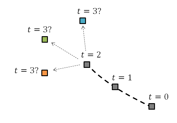
Figure 1. What is the most likely position of the object at t = 3 based on the trajectory so far?
A more advanced example is implemented in the video below, which shows the estimation of the trajectory of a ball using the Kalman filter. The size of the red circle indicates the uncertainty of the prediction for the next step.
Two operations related to normal distribution: convolution and product
The Kalman filter we are dealing with describes all states and actions using the normal distribution.
Also, since the Kalman filter deals with “changes in state over time,” we need to know in advance about the changes in the state represented by the normal distribution. The changes in the state can be expressed through two operations: convolution and product. (A detailed discussion will be done below.)
For a detailed proof of the two operations, please refer to the literature “Products and Convolutions of Gaussian Probability Density Functions”. We only want to confirm the results of these operations.
Since both convolution and product deal with two normal distributions, we want to define each normal distribution function as follows:
\[\mathcal{N}_1(x;\mu_1, \sigma_1^2) = \frac{1}{\sqrt{2\pi \sigma_1^2}}\exp\left(-\frac{(x-\mu_1)^2}{2\sigma_1^2}\right)\] \[\mathcal{N}_2(x;\mu_2, \sigma_2^2) = \frac{1}{\sqrt{2\pi \sigma_2^2}}\exp\left(-\frac{(x-\mu_2)^2}{2\sigma_2^2}\right)\]By the way, from now on, we will use the symbol $\mathcal{N}$ to represent the normal distribution, and when it is written as $\mathcal{N}(x;\mu_1, \sigma_1^2)$, it means that the domain is $x$ and the parameters are $\mu_1, \sigma_1^2$, which represent the mean and variance, respectively.
Convolution of two normal distributions
The first state transition operation to check is the convolution of two normal distributions.
Convolution is an operation defined for any two functions $f(t)$ and $g(t)$ as follows:
\[f(t) \circledast g(t) = \int_{-\infty}^{\infty}f(\tau)g(t-\tau)d\tau\]To explain the formula, convolution can be thought of as a mathematical operator that obtains a new function by multiplying one function and another function that is inverted and shifted, and then integrating it over an interval.
In other words, it can be thought of as obtaining a new function by sliding one function over another and multiplying the resulting values, as shown in the following figure.
A more detailed discussion can be found on Wikipedia (https://en.wikipedia.org/wiki/Convolution).
For the following two normal distributions:
\[\mathcal{N}_1(x;\mu_1, \sigma_1^2)\text{ , }\mathcal{N}_2(x;\mu_2, \sigma_2^2)\notag\]The convolution result is as follows:
\[\mathcal{N}_1 \circledast \mathcal{N}_2 = \mathcal{N}(x; \mu_1+\mu_2, \sigma_1^2 +\sigma_2^2)\]
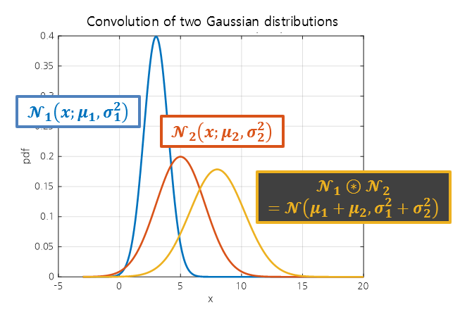
Figure 2. Convolution of two normal distributions.
When convolution is performed, the resulting function also follows a normal distribution, but its mean and variance are calculated as the sum of the means and variances of the two normal distributions used as inputs.
Therefore, when convolution is performed, the variance of the output value always becomes larger than the variances of the two normal distributions used as inputs.
The process of performing convolution on two normal distributions can be seen in the video below.
Product of two normal distributions
The second operation to be used for state transition is the product of two normal distributions.
What happens when we multiply two normal distributions? Surprisingly, the result is also a normal distribution.
If the resulting normal distribution from the multiplication is denoted as
\[\mathcal{N}_{new}(x; \mu_{new}, \sigma_{new}^2)\notag\]then $\mu_{new}$ and $\sigma_{new}^2$ are determined as follows:
\[\mu_{new} = \frac{\mu_1\sigma_2^2 + \mu_2\sigma_1^2}{\sigma_1^2+\sigma_2^2}\] \[\sigma_{new}^2 = \frac{1}{1/\sigma_1^2+1/\sigma_2^2}=\frac{\sigma_1^2\sigma_2^2}{\sigma_1^2 + \sigma_2^2}\]This is illustrated in the following figure.
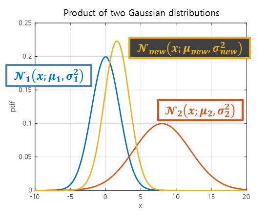
Figure 3. Product of two normal distributions.
From the formulas for $\mu_{new}$ and $\sigma_{new}^2$, we can deduce the following:
First, $\mu_{new}$ is located between $\mu_1$ and $\mu_2$ and closer to the normal distribution with smaller variance.
Also, $\sigma_{new}^2$ can be written as follows:
\[\sigma_{new}^2=\sigma_1^2\frac{\sigma_2^2}{\sigma_1^2 + \sigma_2^2}=\sigma_2^2\frac{\sigma_1^2}{\sigma_1^2 + \sigma_2^2}\]From this, we can confirm that the value of the new $\sigma_{new}^2$ is always smaller than $\sigma_1^2$ or $\sigma_2^2$.
Position Estimation and Movement
In the Kalman filter, the ‘state’ is represented using normal distributions.
In the Kalman filter, both the current position and movement can be represented using normal distributions.
By using normal distributions, we can represent not only the current position or movement, but also the ‘uncertainty’.
For example, suppose we want to measure the position of an object that is most likely at $x=0$ currently.
If we measure the position using two different methods with different degrees of uncertainty, we can represent them using normal distributions with different variances as shown in the following figure.
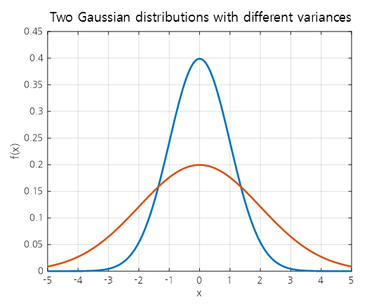
Figure 4. Comparison of two normal distributions with different variances representing the uncertainty of an object's position being at $x=0$.
That is, compared to the blue normal distribution, the orange normal distribution has a higher uncertainty about the object being at $x=0$.
Similarly, we can represent movement using normal distributions. For example, suppose there is an object that will move 4 units to the right in the next step.
However, there is uncertainty about whether the object will move exactly 4 units, so we can represent it as a normal distribution as shown in the following figure.
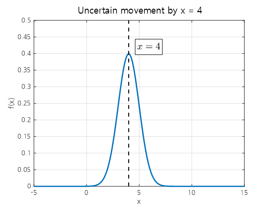
Figure 5. The movement of 4 units to the right can be represented using a normal distribution with uncertainty.
If an object that was initially located at $x=0$ moves $x=4$ to the right at each step, how will its position and uncertainty change at each step?
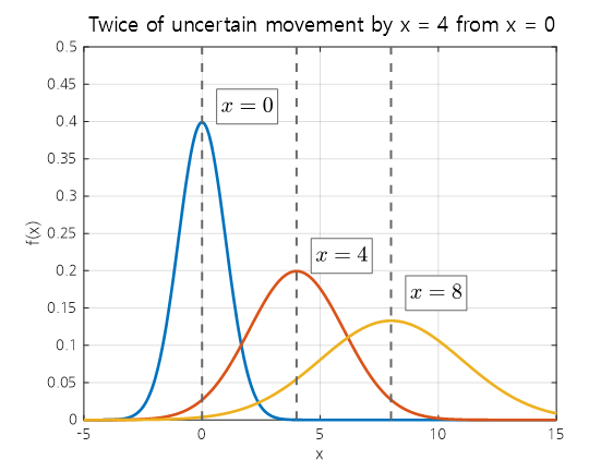
Figure 6. When an object that was located at x=0 is moved twice by x=4, the uncertainty at each position can be represented by the variance of a normal distribution.
It can be observed from the figure that uncertainty increases each time the object moves.
This is because the movement of the object can be obtained by convolving two normal distributions: the normal distribution that represented the object’s original position and the normal distribution that represents the movement.
In summary, the movement of an object can be represented by convolving the normal distribution of the object’s current position and the normal distribution of its movement, and the uncertainty regarding the position increases each time the convolution is performed.
(This is because the uncertainty included in the normal distribution of the movement is added.)
Bayes’ Theorem: Update Rule
Bayes’ theorem is one of the conditional probability rules and is written as follows:
\[P(H|E) = \frac{P(E|H)P(H)}{P(E)}\]Here, H stands for Hypothesis and E stands for Evidence.
The important point in Bayes’ theorem is the relationship between prior probability and posterior probability.
Bayes’ theorem needs to be understood from a different perspective on probability to understand its essence. In Bayesianism, probability refers to the ‘degree of belief’ in a claim. Bayes’ theorem describes an update rule that updates the degree of belief in an existing claim by observing evidence.
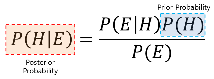
Figure 7. Two important probabilities in Bayes' theorem (prior probability, posterior probability)
Another key point in understanding Bayes’ theorem is to understand that the denominator on the right-hand side of the equation is simply a normalization process that turns the posterior probability value into a ‘probability’.
In other words, no matter how complex Bayes’ theorem may seem, $P(E)$ is just a probability value, and it is simply a normalization process. Therefore, Bayes’ theorem can also be written as follows.
\[P(H|E) = \frac{1}{Z}P(E|H)P(H)\]In other words, the posterior probability is proportional to the product of the prior probability ($P(H)$) and the likelihood ($P(E|H)$).
Operation process of the very simplified Kalman filter
The Kalman filter operates through two processes: Predict and Update.
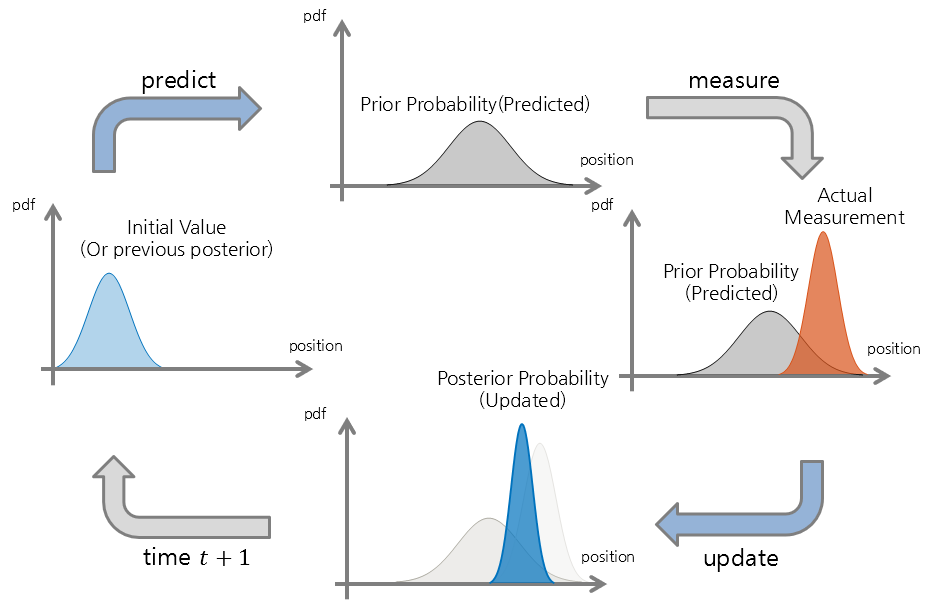
Figure 8. The operation steps of the Kalman filter consist of two processes, Predict and Update.
Predict
The Predict process describes the movement from the current position to the next position.
In other words, it performs the movement from the previous position to the current step. Both the current position and the movement are represented using the normal distribution, as seen in the position estimation and movement section, and the movement process is performed using convolution.
Update
The Update process updates the predicted position calculated through Predict.
Bayes’ theorem and the product of normal distributions are used here, where the updated probability distribution ($P(H|E)$) of the current position is calculated by multiplying the predicted probability distribution ($P(H)$) and the probability distribution of the actual measured position ($P(E|H)$) obtained through measurement.
Using the product of normal distributions, the updated posterior probability distribution can be calculated for the updated current position.
As seen in the process of multiplying normal distributions, the normal distribution as the multiplied result continues to decrease in variance, so assuming a certain law, it is possible to predict with a constant pattern.
In other words, the variance of the posterior probability can converge at a certain value, allowing for prediction at an accurate position that is as precise as the measure.
Operation process of the simple Kalman filter
Figure y.