※ This post was written based on Stanton Glantz’s Primer of biostatistics textbook.
Prerequisites
To better understand the content of this post, it is recommended that you have knowledge of the following:
Motivation
In the previous post on Paired t-test, we looked at the paired t-test, which allows us to compare each subject before and after treatment.
As with the independent t-test, the paired t-test also assumes that the samples come from a population with a normal distribution.
In this post, we will explore Wilcoxon’s signed rank test, the non-parametric version of the paired t-test. As the term “non-parametric” suggests, this test does not make assumptions about normality.
Signed Rank Test
Introduction to the Principles of the Signed Rank Test
The signed rank test can be thought of as an upgrade to the sign test.
The main point is that the data used in the signed rank test is divided into before and after data. Therefore, we can see the difference between before and after treatment by looking at these data.
We will rank the ‘difference’ values and assign a rank that includes a sign.
Then, we will use the sum of the ranks that include the sign as a statistic. As with the t-test or sign test, we will investigate all possible statistics, and see how significant the statistic we obtain is.
Let’s try to understand this in more detail through an example.`
The following figure is an experiment in which the amount of urine was measured before and after administering a diuretic to six people.

Figure 1. Experiment observing changes in urine volume after administering a diuretic to six people.
Source: Primer of Biostatistics 7th ed., Stanton A. Glantz
As shown in Figure 1, to perform a signed rank test, the result of before and after conditions for each subject must be subtracted. Then, the differences are ranked according to their sizes. Note that we do not consider the signs of the differences here. Therefore, if the difference is 100 or -100, they should be considered the same rank.
Once all ranks have been assigned, signs are added to the ranks according to the signs of the differences.
Then, the sum of signed ranks for all individuals can be calculated to obtain the test statistic W at the bottom right of Figure 1.
Now, we need to determine how significant the obtained test statistic W is.
As with the rank sum test, we will simulate all possible combinations of signs and ranks to obtain the distribution of W values. Then, we will determine whether our obtained W value is significantly large or small.
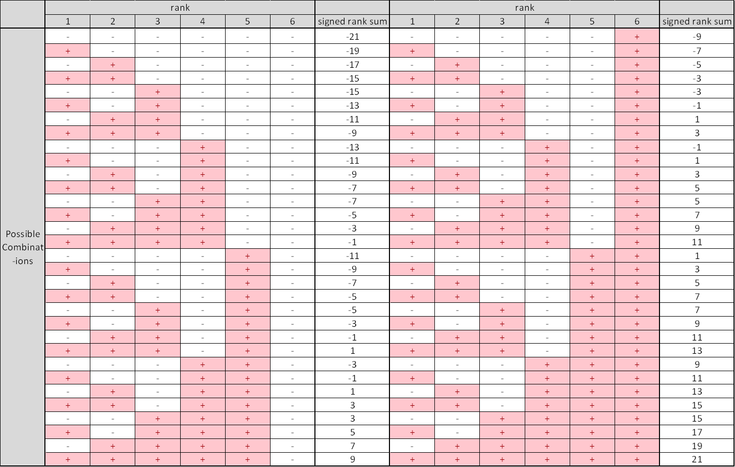
Therefore, let’s calculate the value of W for all possible combinations of + and - signs for the six ranks as shown in the figure below.

Figure 2. Calculation of W values for all possible combinations of six ranks and two signs.
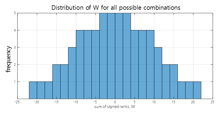
There are a total of $2^6=64$ combinations, and the histogram of the values obtained for $W$ in this case is shown below:

Figure 3. Histogram of all possible combinations of W
By looking at this, we can see that the two on each side (i.e., $W$ is 19 or higher or -19 or lower) account for 4/64 = 0.0625 or 6% of $W$ values.
However, the value of $W$ we obtained is -13, which is greater than -19, the value that represents 6% of both sides. Therefore, we can conclude that the magnitude of $W$ is not large enough to reject the null hypothesis that there is no difference between the two groups.
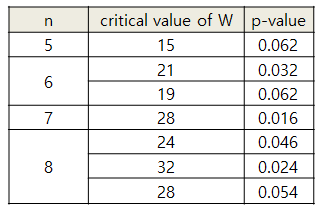
Using this method, we can easily calculate the critical value by computing $W$ for all possible combinations when $n$ is relatively small. Figure 4 shows the significant values of $W$ and the corresponding p-values for $n=5$, $6$, $7$, and $8$.

Figure 4. Significant values of $W$ and p-values for $n=5$ to $8$.
Source: Mosteller F, Rourke R, Sturdy Statistics: Nonparametrics and Order Statistics, Reading, MA: Addison-Wesley; 1973
Normal Approximation of the Signed Rank Test
What if the sample size n is quite large when performing the signed rank test?
If n is greater than or equal to 10, the number of possible combinations can become quite large, as there are $2^n$ possible combinations.
Therefore, we can indirectly obtain the result of the signed rank test through the normal approximation using the same approach as in the sign test.
When n is large, $W$ approximates a normal distribution with the following parameters:
\[\mu_W = 0\] \[\sigma_W = \sqrt{\frac{n(n+1)(2n+1)}{6}}\]Here, $n$ is the number of experimental subjects.
Therefore, we can consider the following variable $Z$, which will follow a normal distribution:
\[Z_W = \frac{W-\mu_W}{\sigma_W}=\frac{W}{\sqrt{[n(n+1)(2n+1)]/6}}\]Similar to the continuity correction in the sign test, $Z_W$ can be adjusted as follows:
\[Z_W = \frac{|W|-1/2}{\sqrt{[n(n+1)(2n+1)]/6}}\]Reference
- Primer of biostatistics, 7th ed., S. Glantz / Ch. 10 Alternatives to Analysis of Variance and the t Test Based on Ranks