Before getting started…
In this article, we will first understand the working principle of the naive Bayes classifier and try to gain additional understanding of the background theory that led to its formula.
Naive Bayes classifier is a type of probabilistic classifier that uses Bayes’ theorem.
To understand the naive Bayes classifier, it is crucial to properly understand the philosophy of Bayes’ theorem rather than just its formula.
To better understand this article, it is recommended to familiarize yourself with the following concepts:
- Theory on likelihood: Introduction to Maximum Likelihood Estimation
In addition, knowing about Bayes’ theorem will also be helpful.
- Contents on Bayes’ Rule: Meaning of Bayes’ Theorem
Finding Probabilistic Basis for Classification
Classification using Prior Knowledge: prior
Let’s consider an example of classifying a sample without any additional information, but with probabilistic background knowledge.
For example, imagine someone brings in a person and asks you to classify whether that person is male or female without any information. How would you think?
If you think that half of the world’s population is male and the other half is female, then you can only make an approximate guess with a 50% probability.
You can only randomly guess one of the two genders.
However, let’s say someone brings in a calico cat and asks you whether it is a female or male cat.
For some unknown reason, calico cats are known to be mostly female due to their sex chromosomes.
In that case, wouldn’t you think that the calico cat is most likely a female?

Figure 1. Calico cats are known to be 99% female due to their sex chromosomes.
As shown above, even without any information (i.e., features) about the test data sample, it is possible to classify the test data sample based solely on prior knowledge, and the probability value that helps with this classification is called prior probability.
By the way, this prior probability can be calculated in advance based on the ratio between classes in the training data in actual data. For example, if class A, B, and C are given in a ratio of 30:30:40 in 100 training data samples, then the prior probability values for each class would be 0.3, 0.3, and 0.4, respectively.
However, in reality, wouldn’t we provide at least some data that would serve as a minimal basis for judgment when classifying data?
Case of adding specific information: likelihood
Let’s consider the problem of determining whether a person is male or female based on their height (i.e., specific information).
Let’s say we know from the given training samples that the height distributions of males and females are different, as shown below. (This distribution modeling can be easily constructed by calculating the mean and variance of the training samples assuming a normal distribution.)
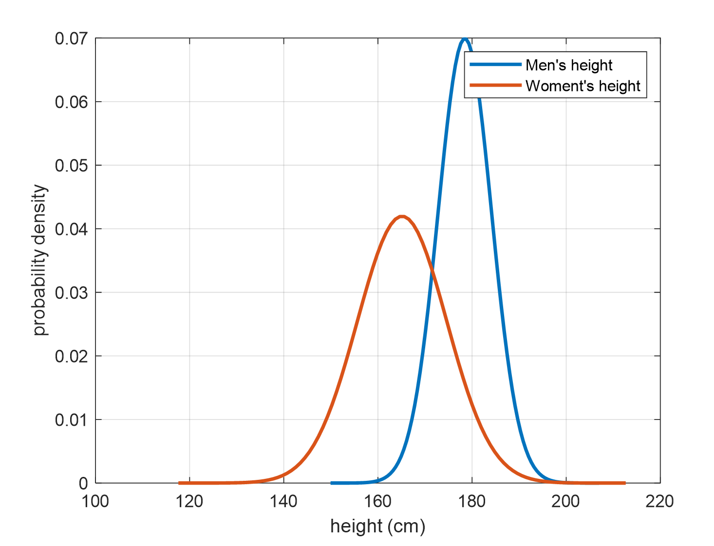
Figure 2. Probability distributions of height for males and females obtained from training samples
Now, let’s say we have a person with a height of 175cm that we want to classify. What can we say about the distribution of our constructed probability density function for 175cm?
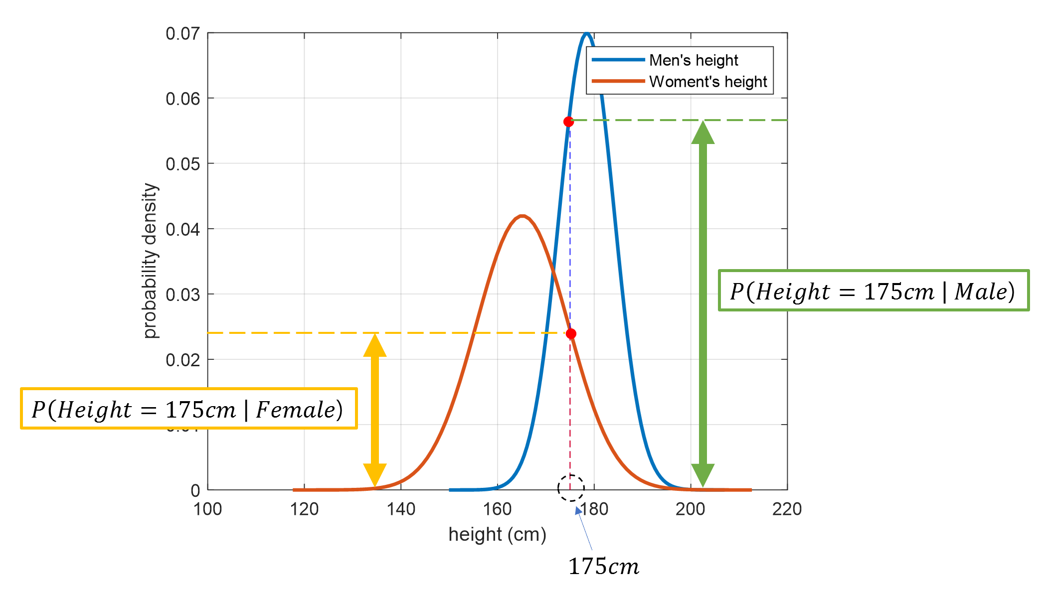
Figure 3. The result of substituting the value of the test data sample into the probability distributions of height for males and females that we have constructed
From the above Figure 3, we can determine the answer. It appears that the probability of the person being male is higher than the probability of the person being female.
The “likelihood contribution” mentioned in the introduction to Maximum Likelihood Estimation is precisely what we mean by “likelihood” in this example, since there is only one feature available.
We can think of this likelihood as follows.
The likelihood of a height being 175cm when judged as male can be expressed as:
\[P(Height=175cm | Gender = Male)\]On the other hand, the likelihood of a height being 175cm when judged as female can be expressed as:
\[P(Height=175cm | Gender = Female)\]From this example, we can also see that the values of likelihood in equation (1) and equation (2) are as follows:
\[P(Height=175cm | Gender = Male) > P(Height=175cm | Gender = Female)\]We can easily understand that equation (3) is a strong evidence for determining that this person is male based on the likelihood comparison.
However, is it enough evidence to determine that this person is male based solely on the likelihood comparison?
Not necessarily.
This is because likelihood is additional information, as mentioned earlier. In other words, it is additional information added to our existing prior knowledge. Therefore, in order to determine whether this person is male or female, we can find the “evidence for determination” by multiplying the likelihood with the prior knowledge in the background.
(In other words, we cannot completely ignore prior knowledge.)
To summarize, the evidence for determining that the person is male, based on the prior knowledge and likelihood, is as follows:
\[P(Gender = Male) \times P(Height=175cm | Gender = Male)\]And the evidence for determining that the person is female, based on the prior knowledge and likelihood, is as follows:
\[P(Gender = Female) \times P(Height=175cm | Gender = Female)\]We can compare these two evidences, obtained by multiplying prior knowledge and likelihood, to determine the gender of the test data person.
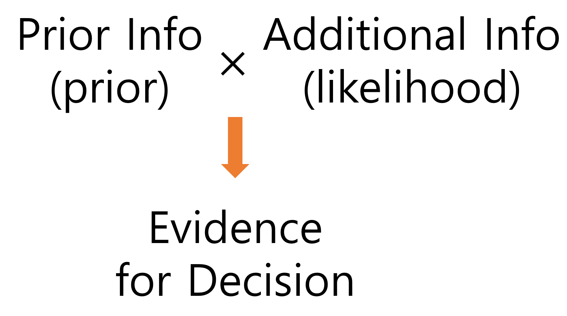
Figure 4. The multiplied value of prior knowledge (prior) and additional information (likelihood) can be used as evidence for decision-making (or judgment) of the given data.
What if more information is added?
If more information is added, such as weight in addition to height, how can we incorporate it into our analysis?
In that case, just like we multiplied and added the additional information to the prior information using the likelihood, we can continue to append the additional information to the posterior.
For example, if we have test data for a person’s weight as 80kg, we can update the evidence for classifying the person as male as follows:
The evidence for classifying the person as male is given by:
\[P(Gender = Male) \times P(Height = 175cm | Gender = Male) \times P(Weight = 80kg | Gender = Male)\]On the other hand, the evidence for classifying the person as female is given by:
\[P(Gender = Female) \times P(Height = 175cm | Gender = Female) \times P(Weight = 80kg | Gender = Female)\]By comparing these two pieces of evidence, we can determine whether the person is male or female.
Introduction to Background Theory
The entire content described above is based on a solid theoretical foundation.
In fact, the explanation using Bayes’ theorem seems to be complicated in mathematical notation, so I moved that content to the later part.
For more information about Bayes’ theorem, refer to the following article:
In this section of the article, we will focus on understanding the process of deriving the ‘evidence’ for decision making through the mathematical derivation of Bayes’ theorem.
Deriving the ‘Evidence’ for Decision Making through Bayes’ Theorem
In fact, what we really want is to determine the class of the given data when we observe this data, and the evidence for decision making can be obtained from probabilities.
In other words, for two classes $c_1, c_2$ and given data $x$, we can determine the class of the data based on the following posterior probabilities:
\[P(c_i | x)\text{ for }i=1, 2\]For example, if $P(c_1 | x) > P(c_2 | x)$, then the label of the sample is classified as $c_1$, otherwise it is classified as $c_2$.
If we express this in a mathematical formula, it would be as follows:
\[P(c_1 | x) >? P(c_2 | x)\]Here, let’s understand $A>?B$ as “Is A greater than B?”
Applying Bayes’ theorem to the equation (9) above, we get:
\[\frac{P(x | c_1)P(c_1)}{p(x)} >? \frac{P(x | c_2)P(c_2)}{p(x)}\]Looking closely at equation (10), we can see that the denominators of the two probabilities being compared are the same.
Therefore, regardless of the value of $p(x)$, the result of the class decision will not change, so we can ignore it.
As a result, we can make a class decision based on the values excluding the denominator in equation (10).
\[P(x | c_1)P(c_1) >? P(x | c_2)P(c_2)\]What if the data has more than one feature?
If we want to make a decision on class $c_i$ based on multiple features $x_1, x_2, \cdots, x_n$, the formula becomes slightly more complex.
In other words, instead of comparing $P(c_i | x)$ for each data, we compare $P(c_i | x_1, x_2, \cdots, x_n)$.
For example, if we have only two classes, $c_1$ and $c_2$, and n features are given, the formula can be written as follows:
\[P(c_1 | x_1, x_2, \cdots, x_n) >? P(c_2 | x_1, x_2, \cdots, x_n)\]If we expand only $P(c_1 | x_1, x_2, \cdots, x_n)$, we get the following:
\[P(c_1 | x_1, x_2, \cdots, x_n) = P(c_1) P(x_1|c_1) P(x_2 | c_1, x_1) P(x_3 | c_1, x_1, x_2) \cdots P(x_n | c_1, x_1, x_2, \cdots x_{n-1})\]Let’s assume that the features are all independently extracted.
(That’s why this type of classifier is called “naive” Bayes.)
Then, for example, $P(x_2 | c_1, x_1)$ can be written as follows:
\[P(x_2 | c_1, x_1) = P(x_2 | c_1)\]This means that the occurrence of $x_1$ does not affect the probability of $x_2$, regardless of whether $x_1$ occurs or not.
So, rewriting equation (13), we have:
\[P(c_1 | x_1, x_2, \cdots, x_n) = P(c_1) P(x_1|c_1) P(x_2 | c_1) P(x_3 | c_1) \cdots P(x_n | c_1) \notag\] \[= P(c_1) \prod_{i=1}^{n}P(x_i | c_1)\]This allows us to derive the ‘evidence for decision’ in equation (6) or (7) using this approach.
In other words, when using a Naive Bayes classifier, the predicted class $\hat{y}$ can be obtained as follows:
\[\hat{y} = argmax_{k\in \lbrace 1, 2, \cdots, k\rbrace}P(c_k)\prod_{i=1}^{n}P(x_i | c_k)\]