Gaussian integration is an integration over the entire range of real numbers for the Gaussian function, and its value is as follows.
\[\int_{-\infty}^{\infty}\exp\left(-x^2\right)dx=\sqrt \pi\]Calculation process of Gaussian integration
First, let’s denote the value of Gaussian integration as $I$.
\[I = \int_{-\infty}^{\infty}\exp\left(-x^2\right)dx\]Then, the square of $I$, denoted as $I^2$, can be thought of as follows.
\[I^2 = \int_{-\infty}^{\infty}exp\left(-x^2\right)dx \int_{-\infty}^{\infty}exp\left(-y^2\right)dy\] \[=\int_{-\infty}^{\infty}\int_{-\infty}^{\infty}exp\left(-x^2\right)exp\left(-y^2\right)dxdy\] \[=\int_{-\infty}^{\infty}\int_{-\infty}^{\infty}exp\left(-(x^2+y^2\right))dxdy\]Now, let’s try changing the Cartesian coordinates to polar coordinates as follows.
\[\begin{cases}x = r\cos\theta \\y = r\sin\theta\end{cases}\]Cartesian coordinates ⇒ Polar coordinates: Modification of integration range
The integration range changes as follows.
\[\begin{cases}-\infty<x<\infty \\-\infty<y<\infty\end{cases} \Rightarrow \begin{cases} 0<r<\infty \\0<\theta<2\pi\end{cases}\]The reason why the integration range changes as shown in Equation (7) is that the range of $x$ and $y$ on the left side of Equation (7) represents the entire range of real numbers.
In order to cover the entire range of real numbers in polar coordinates, the radius ($r$) should vary from $0$ to $\infty$, and the angle should cover a full circle from $0$ to $2\pi$. This is why the integration range changes in polar coordinates.
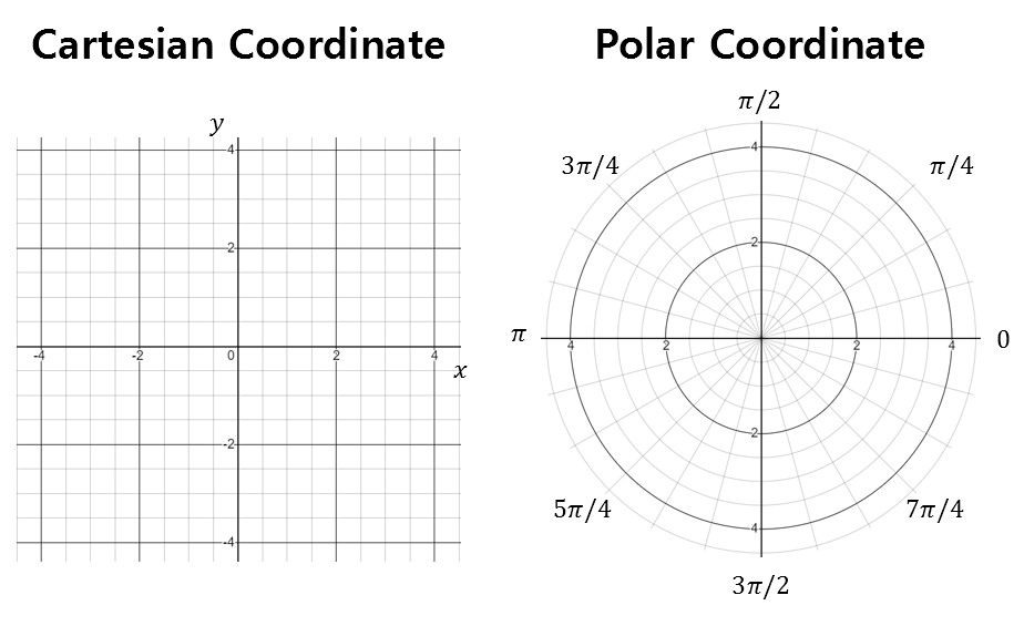
Figure 1. Comparison of Cartesian coordinates and polar coordinates
Cartesian Coordinates to Polar Coordinates: Modifying Infinitesimal Area
The infinitesimal area ($dxdy$) in Equation (5) changes as follows:
\[dxdy \Rightarrow r\space drd\theta\]$dr$ can be thought of as a small displacement in the $r$ direction, and $d\theta$ is a small change in angle. Therefore, $rd\theta$ can be considered as a small displacement in the length of the arc, and ultimately, multiplying the two gives us the infinitesimal area $r\space dr d\theta$.
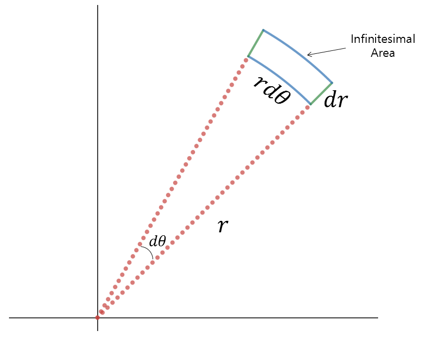
Figure 2. Infinitesimal area in polar coordinates
Let’s continue with the integration.
Considering the two processes above, the integral value of Equation (5) can be written as follows:
\[Equation(5) = \int_{\theta = 0}^{2\pi}\int_{r=0}^{\infty}\exp\left(-r^2\right)rdrd\theta\]This equation can also be written as follows:
\[=\int_{\theta = 0}^{2\pi}d\theta\int_{r=0}^{\infty}\exp\left(-r^2\right)rdr\] \[=2\pi\int_{r=0}^{\infty}\exp\left(-r^2\right)rdr\]Let’s substitute $u = -r^2$.
Then,
\[du = -2rdr\] \[rdr = -\frac{1}{2}du\]Therefore, Equation (11) can be written as follows:
\[Equation(11) = 2\pi\int_{u=0}^{-\infty}-\frac{1}{2}\exp(u)du\] \[=2\pi\cdot\left(-\frac{1}{2}\right)\cdot\left[\exp(u)\right]_{0}^{-\infty}\] \[=2\pi\cdot\left(-\frac{1}{2}\right)\cdot(-1) = \pi\]The result above equals to $I^2$. As the value of $I$ is always positive, we can confirm that
\[I=\int_{-\infty}^{\infty}\exp\left(-x^2\right)dx=\sqrt \pi\]