Gradient Descent is an iterative method that uses the first derivative to find the minimum value of a function.
Let's observe the process of finding the minimum value by adjusting the step size.
Intuitive Meaning of Gradient Descent
Gradient Descent, also known as the steepest descent method, is a method of finding the value of an independent variable that minimizes the function by transforming the value of the independent variable in the direction where the function value decreases.
The steepest descent method is often metaphorically described as follows:
When descending a foggy mountain with no visibility, one can take one step at a time in the direction where the height of the mountain decreases the most.
Purpose and Use of Gradient Descent
Gradient Descent is used to find the minimum value of a function.
One may ask, “Can’t we just find the point where the derivative is 0 to find the minimum or maximum value of a function?”
The main reason for using Gradient Descent instead of finding the points where the derivative is 0 is that:
- The functions we often encounter in real-world analysis are not in closed form or have complex forms (e.g., nonlinear functions), and it is often difficult to calculate the derivative and its roots.
- Gradient Descent can be relatively easily implemented in a computer compared to calculating derivatives in the actual sense.
Additionally,
- When dealing with large amounts of data, using iterative methods such as Gradient Descent can be more computationally efficient in finding solutions.
Derivation of the Formula for Gradient Descent
Gradient descent is a method that uses the gradient (i.e., the slope) of a function to determine where to move the value of $x$ in order to find the minimum value of the function.
If the gradient is positive, it means that as the value of $x$ increases, the value of the function also increases, and conversely, if the gradient is negative, it means that as the value of $x$ increases, the value of the function decreases.
Moreover, a large value of the gradient indicates a steep slope, but on the other hand, it also means that the position of $x$ is far away from the $x$ coordinate corresponding to the minimum/maximum value.
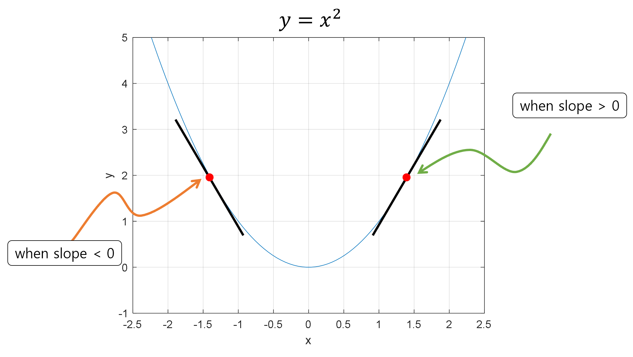
Figure 1. Comparison of positive and negative gradients
Using the Direction Component of the Gradient
Using this information, if at a certain point $x$ the function value increases as $x$ increases (i.e., the sign of the gradient is positive), then $x$ should be moved in the negative direction of the gradient.
On the other hand, if at a certain point $x$ the function value decreases as $x$ increases (i.e., the sign of the gradient is negative), then $x$ should be moved in the positive direction of the gradient.
This logic can be expressed in a formula as follows:
\[x_{i+1} = x_i - \text{step size} \times \text{sign of the gradient}\]Here, $x_{i}$ and $x_{i+1}$ represent the coordinates of $x$ calculated at the $i$-th step and $(i+1)$-th step, respectively.
Now, how should we think about the step size? We can use the magnitude of the gradient to determine it.
Using the Magnitude of the Gradient
The issue with Equation (1) is how to determine the factor called “step size”.
Upon further consideration, we can realize that the absolute value of the derivative coefficient (i.e., the slope or gradient) decreases as we get closer to the local minimum.
In fact, the derivative coefficient also decreases as we get closer to the local maximum, but during the gradient descent process, it is very rare to stay at the local maximum, so we will not consider this issue.
Therefore, if we use a factor that is proportional to the magnitude of the gradient as the step size, we can move a lot when the current value of $x$ is far from the local minimum, and move only a little when we get closer to the local minimum.
In other words, the step size is directly proportional to the gradient value, and the user can adjust the step size according to the situation by modifying the formula.
The adjustment value of the step size is commonly referred to as the “learning rate” and is denoted by $\alpha$.
Therefore, the final formula for updating $x$ can be calculated as follows:
Final Formula
For the function $f(x)$ that we want to optimize, we can express it as follows:
\[x_{i+1} = x_i - \alpha \frac{df}{dx}(x_i)\]
Figure 2. Visualization of gradient descent for function $f(x)$
Image source
When extending this to multivariate functions, we can express it as follows:
\[x_{i+1} = x_i - \alpha \nabla f(x_i)\]The scene below is an example of gradient descent with two variables, which is the process of finding a linear regression model.
You can think of the contour plot on the right side of Figure 3 below as representing the contour lines.
Figure 3. Process of finding the minimum value of the cost function using gradient descent
※ The parameters of the cost function are all normalized for visualization.
Appropriate Step Size
When the step size is large, the advantage is that the distance moved in one step can be large, allowing for rapid convergence. However, if the step size is set too large, the optimization process can progress in the direction of increasing function values without converging to the minimum.
On the other hand, if the step size is too small, it may not diverge, but it takes a long time to find the optimal $x$.
Through the figure below, you can see cases where convergence or divergence does not occur when an inappropriate step size is selected.
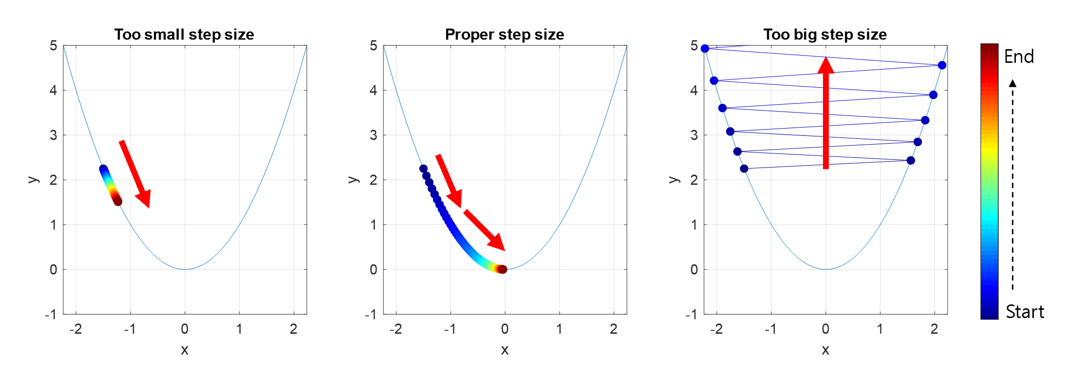
Figure 4. If the step size is too small, the distance moved in each step is too small to converge, and if the step size is too large, it may diverge.
Local Minima Problem
Another issue with gradient descent is the local minima problem. In reality, what we want to find is the global minimum as indicated by the red dot in the figure below. However, due to the random initialization of the gradient descent algorithm, sometimes it can get stuck in local minima and fail to escape from it.
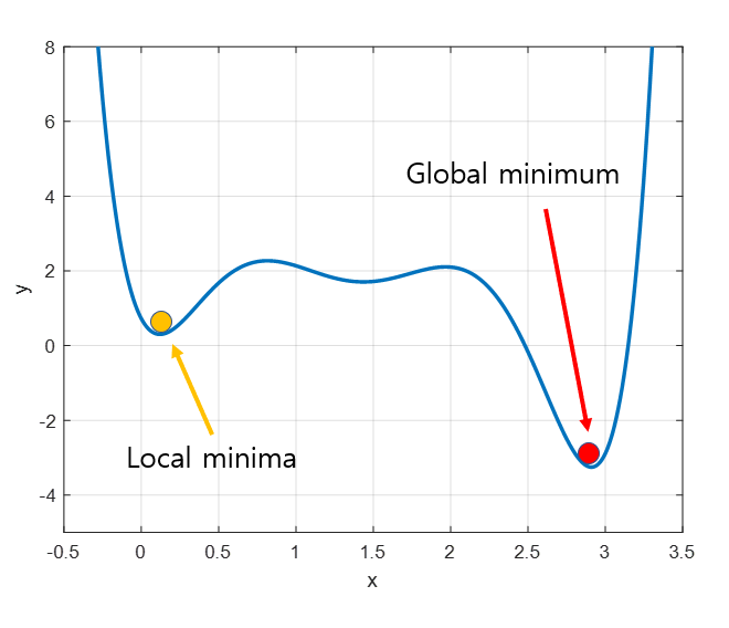
Figure 5. The desired value is the global minimum (red dot), but if the initialization is accidentally incorrect, it may get stuck in local minima (yellow dot).