What Z-Transform is saying: I want to represent the characteristics of a discrete signal (or system) in the Z-plane at once.
Try moving the red marker with your mouse
Definition and Derivation of Z-Transform
| DEFINITION 1. Z-Transform |
|---|
| The transformation of a discrete signal $x[n]$ is called Z-Transform and defined as follows: where $z$ is a complex number |
Z-Transform can be considered as a technique that makes it easy to solve linear difference equations, or more broadly, a generalized form of Discrete Time Fourier Transform (DTFT). This can be best understood by analogy to the relationship between Continuous Time Fourier Transform (CTFT) and Laplace Transform in continuous time domain. In other words, Z-Transform is a general form of DTFT, and DTFT can be considered as a special case of Z-Transform.
Z-Transform and Fourier Transform
By deriving the equation of Z-Transform from the equation of Discrete Time Fourier Transform (DTFT), we can mathematically observe the similarity between DTFT and Z-Transform.
As we know, the equation of DTFT is as follows:
\[x[n] = \int_{-0.5}^{0.5}X_{DTFT}(f) \exp(2\pi fn) df\] \[where\space X_{DTFT}(f) = \sum_{n=-\infty}^{\infty}x[n]\exp(-j2\pi fn)\]Let’s consider the DTFT of $x[n]\exp(-\sigma n)$.
\[\mathfrak{F}\left[x[n]\exp(-\sigma n)\right] = \sum_{n = -\infty}^{\infty} x[n] \exp\left(-(\sigma n + j 2\pi fn)\right)\]By substituting $2\pi f = \omega$, equation (4) can be written as follows:
\[Equation (4) \Rightarrow \sum_{n = -\infty}^{\infty}x[n] \exp\left(-(\sigma+j\omega)n\right)\]Let’s define a complex number $z$ as follows.
\[z = \exp(-(\sigma + j \omega))\]Then, Equation (5) can be written as follows.
\[Equation (5) \Rightarrow \sum_{n=-\infty}^{\infty}x[n]z^{-n}\]This derivation demonstrates the relationship between Z-Transform and DTFT. Furthermore, this derivation illustrates how similar Z-Transform and DTFT are to the relationship between Laplace Transform and CTFT. DTFT is a special case of Z-Transform where the radius of the circle is 1, which is equivalent to taking Z-Transform with $z = \exp\left(-(\sigma + j\omega)\right)$.
One slight difference from Laplace Transform is that in Laplace Transform, $s=\sigma+j\omega$, whereas in Z-Transform, $z = \exp\left(-(\sigma + j\omega)\right)$. This seems to be due to conventional reasons or ideas adopted by developers. Moreover, this slight difference in how $s$ and $z$ are defined leads to differences in determining the stability of the s-plane and z-plane.
Z-Transform and Laplace Transform
Z-Transform can be considered as the discrete-time version of Laplace Transform.
Let’s obtain Z-Transform by sampling the time in the equation of Laplace Transform.
For a continuous-time signal $x(t)$, Laplace Transform is defined as follows.
\[\mathfrak{L}\left[x(t)\right] = X(s) = \int_{0^{-}}^{\infty}x(t) e^{-st}dt\]To sample the continuous-time signal $x(t)$ in time, let’s substitute $t\rightarrow nT$ for a sampling period $T$.
In other words,
\[X(s) = \int_{0^{-}}^{\infty}x(t) e^{-st}dt \big |_{t\rightarrow nT}\]After this process, $x(nT)$ can be viewed as a discrete-time signal. Therefore,
\[X(z) = \sum_{n=0}^{\infty}x(nT)e^{-snT}\]Substituting $z = e^{sT}$,
\[Equation (10) \Rightarrow \sum_{n=0}^{\infty}x[n]z^{-n}\]Through this derivation, we can confirm that Laplace Transform and Z-Transform are mathematically related. In conclusion, Laplace Transform and Z-Transform are techniques to characterize the properties of systems, with differences in how they define complex numbers.
The s-plane and z-plane have the following morphological relationship.
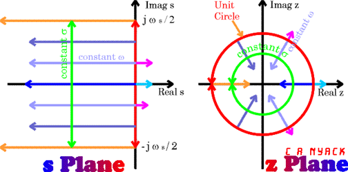
Figure 1. Relationship between s-plane and z-plane. The z-plane has a shape that resembles a folded version of the s-plane.
In Figure 1, in the s-plane, poles should be located to the left of the vertical axis for the system to be stable, while in the z-plane, poles should be located inside the unit circle for the system to be stable.
Applications of Z-Transform
Z-Transform can be used for analysis of discrete-time systems.
Similar to how Laplace Transform is used for continuous-time systems, Z-Transform can be used for analysis of discrete-time systems. In Z-Transform, by substituting $z = \exp(j\omega)$ into the discrete-time transfer function, we can obtain the frequency response of the system. For example, for an AR (AutoRegressive) system given by $y[n] = 0.5 y[n-1] + x[n]$, when we perform Z-Transform, we get:
\[Y(z) = 0.5 \times z^{-1} \times Y(z) + X(z)\] \[\therefore Y(z)(1-0.5\times z^{-1}) = X(z)\] \[H(z) = \frac{Y(z)}{X(z)} = \frac{1}{1-0.5 \times z^{-1}}\]Here, to obtain the frequency response, we substitute $z = \exp(j\omega)$, which gives us:
\[H(z)|_{z = \exp(j\omega)} = H(e^{j\omega}) = \frac{1}{1-0.5e^{-j\omega}}\]As a result, we can plot the frequency response as shown in Figure 2.
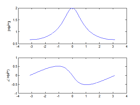
Figure 2. Bode plot of a first-order AR system obtained through Z-Transform.
From the plot, we can see that the system exhibits the characteristics of a low-pass filter.