Prerequisites
To understand this post well, we recommend that you have knowledge of the following:
Invariance and Variability of Vectors
In the basic operations of vectors, we explained that a vector is both “something like an arrow” and “a list of numbers in order.”
The figure below explains both the invariance and variability of vectors. Even if the coordinate system changes, the red arrow remains unchanged (invariance). However, the coordinates of the vector seen through another coordinate system have changed from (3, 4) to (3.6, 3.4) (variability).
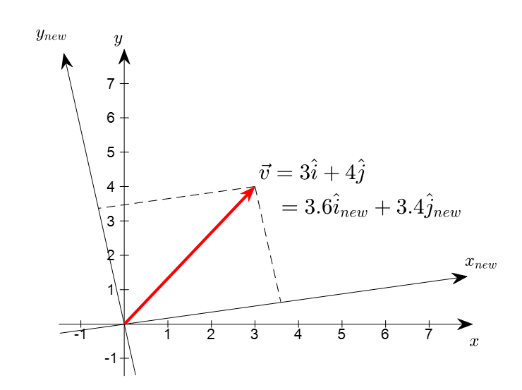
Figure 1. Transformation of coordinate system and vector. When the coordinate system changes, the vector does not change, but the components of the vector do change.
In this post, we will explore how to represent the original vector in a new way when the coordinate system representing the vector changes.
Introduction of a New Basis = A New Coordinate System
Representation of coordinates using the standard basis
When representing a point (i.e., vector) on the Cartesian plane, which is the coordinate system we usually use, we use the Cartesian coordinate.
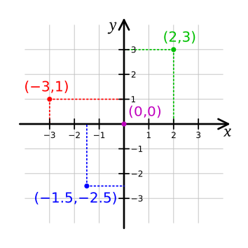
Figure 2. Coordinate plane on 2-dimensional real space of the Cartesian coordinate system
Image source: Wikipedia, Cartesian coordinate system
In the general Cartesian coordinate system, we use the basis vectors that point to $(1,0)$ and $(0,1)$, respectively, and write them as:
\[\hat{i} = \begin{bmatrix}1 \\0 \end{bmatrix}\]and
\[\hat{j} = \begin{bmatrix}0\\1\end{bmatrix}\]In other words, a basis vector can be thought of as determining the length of one unit of horizontal and vertical scales that make up the coordinate system.
Moreover, any arbitrary point on a Cartesian coordinate system, say the point (2,3), can be expressed as a linear combination of two basis vectors, which means that
\[\begin{bmatrix}2\\3 \end{bmatrix} = 2\begin{bmatrix}1\\0 \end{bmatrix} + 3\begin{bmatrix}0\\1 \end{bmatrix} = 2\hat{i} + 3\hat{j}\]Here, we define a term. From now on, let’s call the basis vectors ($\hat{i}, \hat{j}$) of Cartesian coordinate system the standard basis.
Coordinate representation using a new basis
If we construct a coordinate system using a completely new basis instead of the standard basis, how can we represent an arbitrary vector in this new basis?
Let’s consider a set of new basis vectors as follows:
\[\mathcal{B} = \left\lbrace \vec{b_1}, \vec{b_2} \right\rbrace = \left\lbrace\begin{bmatrix}1 \\ 1\end{bmatrix}, \begin{bmatrix}-1 \\ 1\end{bmatrix}\right\rbrace\]
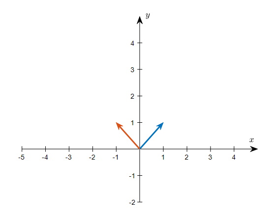
Figure 3. The two basis vectors of an arbitrary new basis vector set $\mathcal{B}$
Using the basis set $\mathcal{B}$, let’s think about a new coordinate system and represent an arbitrary vector using the new basis.
For example, let’s consider the vector (2,2) represented using the standard basis.
If we simultaneously consider the original coordinate system and the new coordinate system, it will be as shown in Figure 4 below.
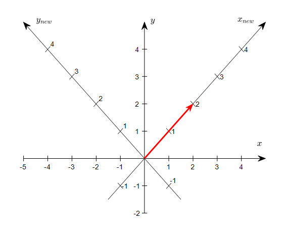
Figure 4. Observations of the vector (2,2) represented using the standard basis in the original coordinate system and the new coordinate system
As shown in Figure 4, it seems sufficient to represent the coordinate of (2,2) in the new coordinate system as (2,0), instead of (2,2) represented using the standard basis.
In the future, when the basis changes, let’s indicate the name of the vector set that serves as the basis as a subscript when representing vectors.
For instance, a (2,2) vector represented in the standard basis is expressed as
\[\begin{bmatrix}2\\ 2\end{bmatrix}_{\mathcal{E}}\]and a vector (1,0) represented based on a new basis $\mathcal{B}$ is written as
\[\begin{bmatrix}2\\ 0\end{bmatrix}_{\mathcal{B}}\]as seen in Figure 4, we can see that the two vector representations are different representations of the same vector.
\[\begin{bmatrix}2\\ 2\end{bmatrix}_{\mathcal{E}}, \begin{bmatrix}2\\ 0\end{bmatrix}_{\mathcal{B}}\]In other words, the above equation can be interpreted as follows.
$\Rightarrow$ In the coordinate system made with basis $\mathcal{B}$, (2,0) can be written as (2,2) in the standard coordinate system.
However, how can we obtain the coordinate value of (2,0) expressed with the basis $\mathcal{B}$ in equation (6)?
Suppose we express the original coordinates (2,2) in the standard coordinate system using the basis vectors of $\mathcal{B}$ and the coordinates expressed using the basis $\mathcal{B}$ are $(k_1, k_2)$.
In other words, the standard coordinate (2,2) and the coordinate expressed using the new basis $(k_1, k_2)$ should satisfy the following relationship.
\[\begin{bmatrix}2\\2\end{bmatrix}=k_1\begin{bmatrix}| \\ b_1 \\ |\end{bmatrix}+k_2\begin{bmatrix}| \\ b_2 \\ |\end{bmatrix}\]As we can see from the above equation, we can rewrite the right side of the equation using the ‘linear combination of column vectors’ interpretation of matrix multiplication, which we saw in another post about a different perspective on matrix multiplication, as follows.
\[\begin{bmatrix}2\\2\end{bmatrix} = \begin{bmatrix}| & | \\ b_1 & b_2 \\ | & |\end{bmatrix}\begin{bmatrix}k_1\\k_2\end{bmatrix}\]Since the basis vectors of $\mathcal{B}$ given to us are as follows,
\[\mathcal{B} = \left\lbrace\begin{bmatrix}1 \\ 1\end{bmatrix}, \begin{bmatrix}-1 \\ 1\end{bmatrix}\right\rbrace\]we can obtain (2,0) by finding $k_1$ and $k_2$ that satisfy
\[\begin{bmatrix}2\\2\end{bmatrix} = \begin{bmatrix}1 & -1 \\1 & 1\end{bmatrix}\begin{bmatrix}k_1\\k_2\end{bmatrix}\] \[\therefore \begin{bmatrix}k_1\\k_2\end{bmatrix}=\begin{bmatrix}1 & -1 \\ 1 & 1\end{bmatrix}^{-1}\begin{bmatrix}2\\2\end{bmatrix} = \begin{bmatrix}2\\0\end{bmatrix}\]When we generalize this result, for an arbitrary vector in the standard coordinate system, we can obtain the coordinates in a coordinate system composed of an arbitrary basis $\mathcal{C}$ as follows:
Let $x$ be an arbitrary vector in the standard coordinate system.
\[x=\begin{bmatrix}x_1 \\ x_2\end{bmatrix}_{\mathcal{E}}\]Let’s consider the basis $\mathcal{C}$ as follows:
\[\mathcal{C}=\left\lbrace\begin{bmatrix}| \\ c_1 \\ |\end{bmatrix}, \begin{bmatrix} | \\ c_2 \\ | \end{bmatrix}\right\rbrace\]Let $y$ be the coordinates of $x$ in the coordinate system composed of the basis $\mathcal{C}$ as follows:
\[y=\begin{bmatrix}y_1\\y_2\end{bmatrix}_{\mathcal{C}}\]Then, we can consider the following relationship:
\[\begin{bmatrix}x_1\\x_2\end{bmatrix}_{\mathcal{E}} = \begin{bmatrix}| & | \\ c_1 & c_2 \\ | & |\end{bmatrix}\begin{bmatrix}y_1\\y_2\end{bmatrix}_{\mathcal{C}}\]Transformation between arbitrary bases
Let’s consider two bases $\mathcal{B}=\lbrace v_1, v_2\rbrace$ and $\mathcal{C}=\lbrace w_1, w_2\rbrace$ in the two-dimensional real space $\Bbb{R}^2$.
Since all vectors in $\Bbb{R}^2$ can be represented as linear combinations of $v_1$ and $v_2$, they can be expressed as follows:
\[w_1 = a v_1 + b v_2\] \[w_2 = c v_1 + d v_2\]
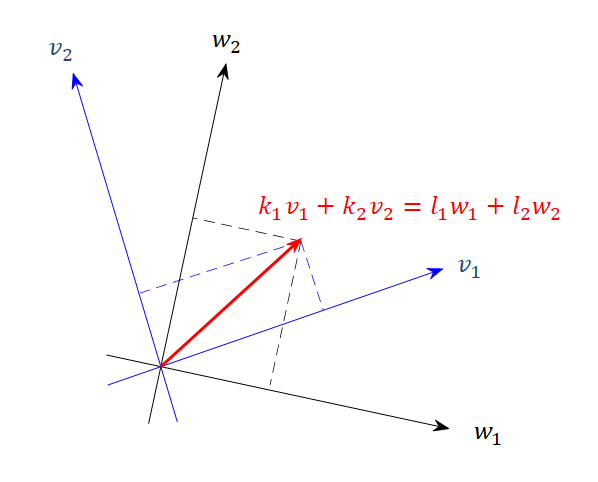
Figure 5.
In Figure 5, if we express vector $v=l_1 w_1 + l_2 w_2$ in terms of $v_1$ and $v_2$, then
\[v = l_1 w_1 + l_2 w_2\] \[=l_1(a v_1 + b v_2) + l_2 (cv_1 +dv_2)\] \[=(a l_1 + cl_2)v_1 + (bl_1 + d l_2)v_2\] \[=k_1v_1 + k_2v_2\]Therefore, using coordinate vectors and matrices,
\[[v]_{\mathcal{B}} = \begin{bmatrix}k_1 \\ k_2\end{bmatrix} = \begin{bmatrix}al_1 + cl_2 \\ bl_1 + dl_2\end{bmatrix} = \begin{bmatrix}a & c \\ b & d\end{bmatrix}\begin{bmatrix}l_1 \\ l_2\end{bmatrix}=\begin{bmatrix}a & c \\ b & d\end{bmatrix}[v]_{\mathcal{C}}\]can be said.
The matrix that changes the representation of vector $v$ in basis $\mathcal{C}$,
\[[v]_{\mathcal{C}}\]to the representation in basis $\mathcal{B}$,
\[[v]_{\mathcal{B}}\]is called the change-of-basis matrix or transition matrix.