This post is written based on the content provided by ZyBooks in ENG 006: Engineering Problem Solving at the University of California Davis.
Simultaneous Equations and Matrices
Solutions to Simultaneous Equations
Let’s revisit the method for solving simultaneous equations that we learned in middle school.
Consider the following set of simultaneous equations:
\[\begin{cases}2x+3y=1 \\ 4x + 7y=3\end{cases}\]To find the solutions to this set of simultaneous equations, we need to eliminate one variable from either the top or bottom equation.
Let’s multiply the top equation by 2 and subtract it from the bottom equation:
We redefine the bottom equation as $r_2$ and perform the following transformation:
\[r_2 \rightarrow r_2 - 2 r_1\]Then, we get:
\[4x+7y - 2(2x+3y)=3 - 2\times 1 = 1\] \[\Rightarrow (4x-4x)+(7y-6y)=y=1\]Thus, we know that $y=1$. We can substitute this value of $y$ into the first equation to obtain:
\[2x+3(1)=1 \Rightarrow x = -1\]Through this process, we can learn that there are three skills we can use to solve simultaneous equations:
- Multiplying both sides of an equation by a number
- Adding two different equations together
- Changing the order of the equations
Representation of Systems of Equations using Matrices
However, if we think about it, we can also represent systems of equations using matrices.
The system of equations in equation (1) can be expressed as follows:
\[\begin{bmatrix}2 & 3 \\ 4 & 7\end{bmatrix}\begin{bmatrix}x\\y\end{bmatrix}=\begin{bmatrix}1\\3\end{bmatrix}\]Alternatively, we can express it as follows, omitting the variables $x$ and $y$:
In the equation represented by the matrix above,
\[A=\begin{bmatrix}2 & 3 \\ 4 & 7\end{bmatrix}\]and
\[b = \begin{bmatrix}1\\3\end{bmatrix}\]We can combine these two matrices side by side and write them as $[A|b]$:
\[[A|b]=\left[\begin{array}{cc|c}2 & 3 & 1 \\ 4 & 7 & 3\end{array}\right]\]This form of the matrix is called an augmented matrix.
The long vertical line in the augmented matrix is just a visual aid and can be treated like a regular $2\times 3$ matrix.
In conclusion, we can solve systems of equations by treating each row of the augmented matrix as an individual equation.
Now, we may understand that we can represent systems of equations using matrices, but is there a reason to use matrices that seem to be even more complicated?
The reason is to solve systems of equations using computers.
To do this, we need to be able to represent the operations corresponding to the “three skills” described earlier in terms of computer operations.
As we saw in another perspective on matrix multiplication, when multiplying two matrices, the left matrix acts as an operator, while the right matrix acts as an operand.
In other words, for any arbitrary matrices $A$ and $B$, $A$ performs the operation and $B$ acts as the operand in the operation $AB$.
Similarly, for the matrix $(A|b)$, we can think of an operator matrix that applies the skills of the system of equations mentioned earlier, and multiplying this matrix by $(A|b)$ allows us to perform “elementary row operations” on the rows of the augmented matrix.
We call a matrix that performs elementary row operations as an elementary matrix, which can be said to have the function of performing elementary row operations. If we can come up with such matrices, we can easily solve systems of equations through matrix multiplication using a computer. If you can think of such matrices, we can easily solve systems of equations through matrix multiplication using a computer.
Elementary matrices
In solving systems of equations, there are three elementary row operations:
- Row multiplication
- Row switching
- Row addition
An elementary matrix performs one of these operations on the rows of a matrix that it is multiplied with. If the matrix being multiplied has dimensions $m\times n$, then the elementary matrix must have dimensions $m\times m$ in order for the matrix size to be maintained after the operation.
An elementary matrix can be obtained by modifying a $m\times m$ identity matrix $I_m$, either by changing a single entry or by permuting rows.
Let’s consider the form of elementary matrices for each operation.
Row multiplication
The elementary matrix for row multiplication has the form:
\[I=\begin{bmatrix}1&0&0\\0&1&0\\ 0&0&1\end{bmatrix} \rightarrow E=\begin{bmatrix}1 & 0 & 0 \\ 0 & \color{red}{s} & 0 \\ 0 & 0 & 1\end{bmatrix}\]That is, it is obtained by replacing one of the entries of the identity matrix with a non-zero scalar $s$. The matrix $E$ shown above changes the second row by multiplying it by the scalar $s$. This operation can be expressed as $r_2 \rightarrow sr_2$. When applied to an arbitrary $3\times 4$ matrix $A$, this operation results in the following transformation:
\[EA = \begin{bmatrix}1 & 0 & 0 \\ 0 & \color{red}{s} & 0 \\ 0 & 0 & 1\end{bmatrix} \begin{bmatrix} a_{11} & a_{12} & a_{13} & a_{14}\\ \color{red}{a_{21}} & \color{red}{a_{22}} & \color{red}{a_{23}} & \color{red}{a_{24}} \\ a_{31} & a_{32} & a_{33} & a_{34} \end{bmatrix} =\begin{bmatrix} a_{11} & a_{12} & a_{13} & a_{14}\\ \color{red}{sa_{21}} & \color{red}{sa_{22}} & \color{red}{sa_{23}} & \color{red}{sa_{24}} \\ a_{31} & a_{32} & a_{33} & a_{34} \end{bmatrix}\]Additionally, it is worth considering that the inverse operation for the operation of row multiplication, which multiplies a row by $s$, is performing the operation of multiplying the same row by $1/s$. As shown below, the inverse matrix for the operation of multiplying the second row by $s$ is:
\[E^{-1}=\begin{bmatrix}1 & 0 & 0 \\ 0 & \color{red}{1/s} & 0 \\ 0 & 0 & 1\end{bmatrix}\]This represents the inverse of the elementary matrix corresponding to the row multiplication operation.
In other words,
\[EE^{-1}=E^{-1}E=I\] \[\Rightarrow \begin{bmatrix}1 & 0 & 0 \\ 0 & \color{red}{s} & 0 \\ 0 & 0 & 1\end{bmatrix}\begin{bmatrix}1 & 0 & 0 \\ 0 & \color{red}{1/s} & 0 \\ 0 & 0 & 1\end{bmatrix}=\begin{bmatrix}1 & 0 & 0 \\ 0 & \color{red}{1/s} & 0 \\ 0 & 0 & 1\end{bmatrix}\begin{bmatrix}1 & 0 & 0 \\ 0 & \color{red}{s} & 0 \\ 0 & 0 & 1\end{bmatrix}=\begin{bmatrix}1&0&0\\0&1&0\\ 0&0&1\end{bmatrix}\]Row switching
Row switching can be obtained by swapping rows of the identity matrix. For example, if we want to perform an operation that swaps the second and third rows, we can consider the following matrix:
\[I=\begin{bmatrix} 1 & 0 & 0 \\ \color{red}{0} & \color{red}{1} & \color{red}{0} \\\color{blue}{0} & \color{blue}{0} & \color{blue}{1}\end{bmatrix}\rightarrow P_{32}= \begin{bmatrix} 1 & 0 & 0 \\ \color{blue}{0} & \color{blue}{0} & \color{blue}{1}\\ \color{red}{0} & \color{red}{1} & \color{red}{0}\end{bmatrix}\]The matrix that performs row switching among basic matrices is also called a permutation matrix, and the symbol is denoted by $P$. Conventionally, the numbers of the two rows to be exchanged are written as $P_{ij}$, specifying which two rows are to be swapped.
For example, if you multiply a $3\times 4$ matrix by $P_{32}$, it results in the following.
\[P_{32}A=\begin{bmatrix} 1 & 0 & 0 \\ \color{blue}{0} & \color{blue}{0} & \color{blue}{1}\\ \color{red}{0} & \color{red}{1} & \color{red}{0}\end{bmatrix} \begin{bmatrix} a_{11} & a_{12} & a_{13} & a_{14}\\ \color{red}{a_{21}} & \color{red}{a_{22}} & \color{red}{a_{23}} & \color{red}{a_{24}} \\ \color{blue}{a_{31}} & \color{blue}{a_{32}} & \color{blue}{a_{33}} & \color{blue}{a_{34}} \end{bmatrix} = \begin{bmatrix} a_{11} & a_{12} & a_{13} & a_{14}\\ \color{blue}{a_{31}} & \color{blue}{a_{32}} & \color{blue}{a_{33}} & \color{blue}{a_{34}}\\ \color{red}{a_{21}} & \color{red}{a_{22}} & \color{red}{a_{23}} & \color{red}{a_{24}} \end{bmatrix}\]In addition, it is worth noting that the inverse of a permutation matrix, which switches the order of rows, is itself. This is quite obvious because to undo an operation that swaps the first and third rows, you only need to swap them back again.
In other words, for the following matrix:
\[P_{31}=\begin{bmatrix}0 & 0& \color{red}{1} \\ 0 & 1 & 0 \\ \color{blue}{1} & 0 & 0\end{bmatrix}\]its inverse is
\[P^{-1}_{31}=\begin{bmatrix}0 & 0& \color{red}{1} \\ 0 & 1 & 0 \\ \color{blue}{1} & 0 & 0\end{bmatrix}\]Row-addition matrices
Lastly, another basic row operation is adding one row to another and replacing the result in a given row. This operation can be expressed mathematically as follows: for example, adding row 1 multiplied by a scalar $s$ to row 2 leads to the following result.
\[\begin{bmatrix} \color{blue}{a_{11}} & \color{blue}{a_{12}} & \color{blue}{a_{13}} & \color{blue}{a_{14}}\\ \color{red}{a_{21}} & \color{red}{a_{22}} & \color{red}{a_{23}} & \color{red}{a_{24}} \\ a_{31} & a_{32} & a_{33} & a_{34} \end{bmatrix} \rightarrow \begin{bmatrix} a_{11} & a_{12} & a_{13} & a_{14}\\ \color{red}{a_{21}} \color{black}{+} \color{blue}{sa_{11}} & \color{red}{a_{22}} \color{black}{+} \color{blue}{sa_{12}} & \color{red}{a_{23}} \color{black}{+} \color{blue}{sa_{13}} & \color{red}{a_{24}} \color{black}{+} \color{blue}{sa_{14}}\\ a_{31} & a_{32} & a_{33} & a_{34} \end{bmatrix}\]Let’s consider a matrix $E$ that performs the operation described above. If we denote the matrix before and after the operation as $A$ and $B$, respectively, we can think of the matrix $E$ as acting on the matrix $A$ as follows.
\[I=\begin{bmatrix}1 & 0 & 0 \\ \color{red}{0} & \color{red}{1} & \color{red}{0} \\ 0 & 0 & 1\end{bmatrix}\rightarrow E = \begin{bmatrix}1 & 0 & 0 \\ \color{red}{s} & 1 & 0 \\ 0 & 0 & 1\end{bmatrix}\] \[EA=\begin{bmatrix}1 & 0 & 0 \\ \color{blue}{s} & 1 & 0 \\ 0 & 0 & 1\end{bmatrix}\begin{bmatrix} \color{blue}{a_{11}} & \color{blue}{a_{12}} & \color{blue}{a_{13}} & \color{blue}{a_{14}}\\ \color{red}{a_{21}} & \color{red}{a_{22}} & \color{red}{a_{23}} & \color{red}{a_{24}} \\ a_{31} & a_{32} & a_{33} & a_{34} \end{bmatrix}=\begin{bmatrix} a_{11} & a_{12} & a_{13} & a_{14}\\ \color{red}{a_{21}} \color{black}{+} \color{blue}{sa_{11}} & \color{red}{a_{22}} \color{black}{+} \color{blue}{sa_{12}} & \color{red}{a_{23}} \color{black}{+} \color{blue}{sa_{13}} & \color{red}{a_{24}} \color{black}{+} \color{blue}{sa_{14}}\\ a_{31} & a_{32} & a_{33} & a_{34} \end{bmatrix}\]Let’s think about how this matrix E performs row-addition operations.
First, one thing to consider is that the operation performed using each row of the matrix E affects each row of the output matrix.
In terms of visualization,
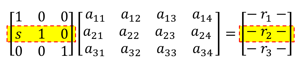
Figure 1. Each row of the matrix being multiplied on the left affects each row of the resulting matrix.
Furthermore, each element of each row of the matrix E being multiplied on the left represents how much weight should be given to each row of the operand matrix.
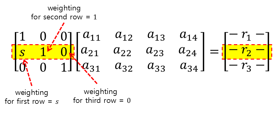
Figure 2. What the elements in each row of the matrix performing the operation represent
Therefore, performing a row addition operation on the output matrix means that the following occurs:
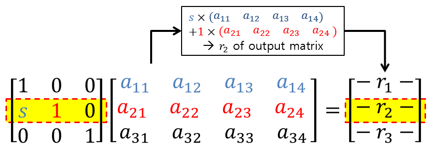
Figure 3. What the elements in each row of the matrix performing the operation represent
By using row addition operations in this way, we can eliminate specific elements as 0, as shown in the following matrix A:
\[A=\begin{bmatrix}\color{blue}{1} & 2 & 3 & 4 \\ \color{red}{1} & -1 & -2 & 2 \\ 0 & 3 & 2 & 1\end{bmatrix}\]To make the first element of the second row 0, we can use the elementary matrix as follows: 2nd row = 2nd row - 1st row.
\[EA = \begin{bmatrix}1 & 0& 0\\ \color{blue}{-1} & 1 & 0 \\ 0 & 0 & 1\end{bmatrix}\begin{bmatrix}\color{blue}{1} & 2 & 3 & 4 \\ \color{red}{1} & -1 & -2 & 2 \\ 0 & 3 & 2 & 1\end{bmatrix}= \begin{bmatrix}\color{blue}{1} & 2 & 3 & 4 \\ \color{red}{0} & -3 & -5 & -2 \\ 0 & 3 & 2 & 1\end{bmatrix}\]Additionally, one can consider the inverse operation for the operation of adding rows to each other, which is multiplying by $-s$ and then adding back.
For example, for the following matrix,
\[E=\begin{bmatrix}1 & 0 & 0 \\ \color{red}{s} & 1 & 0 \\ 0 & 0 & 1\end{bmatrix}\]the inverse matrix is
\[E^{-1}=\begin{bmatrix}1 & 0 & 0 \\ \color{red}{-s} & 1 & 0 \\ 0 & 0 & 1\end{bmatrix}\]Therefore,
\[E^{-1}E=I\] \[=\begin{bmatrix}1 & 0 & 0 \\ \color{red}{-s} & 1 & 0 \\ 0 & 0 & 1\end{bmatrix}\begin{bmatrix}1 & 0 & 0 \\ \color{red}{s} & 1 & 0 \\ 0 & 0 & 1\end{bmatrix}=\begin{bmatrix}1&0&0\\0&1&0\\0&0&1\end{bmatrix}\]Solving systems of equations using elementary matrices
Let’s use elementary matrices to solve the system of equations we saw at the beginning and verify the results by implementing it directly in MATLAB.
\[\begin{cases}2x+3y=1 \\ 4x + 7y=3\end{cases}\] \[[A|b]=\left[\begin{array}{cc|c}2 & 3 & 1 \\ 4 & 7 & 3\end{array}\right]\]To eliminate the term for $x$ in the second equation, let’s perform the following operation:
\[r_2\rightarrow r_2 - 2r_1\]Let’s perform a row addition operation to do this. To do this, let’s multiply the following elementary matrix on the left side of the augmented matrix:
\[E_1=\begin{bmatrix}1&0\\-2&1\end{bmatrix}\] \[\Rightarrow E_1[A|b]=\begin{bmatrix}1&0\\-2&1\end{bmatrix}\left[\begin{array}{cc|c}2 & 3 & 1 \\ 4 & 7 & 3\end{array}\right]\] \[=\left[\begin{array}{cc|c}2 & 3 & 1 \\ 0 & 1 & 1\end{array}\right]\]Now, to eliminate the second element $3$ in the first row, let’s perform the following operation:
\[r_1\rightarrow r_1 - 3r_2\]Let’s multiply the following elementary matrix to do this:
\[E_2=\begin{bmatrix}1&-3\\0&1\end{bmatrix}\] \[\Rightarrow \begin{bmatrix}1&-3\\0&1\end{bmatrix}\left[\begin{array}{cc|c}2 & 3 & 1 \\ 0 & 1 & 1\end{array}\right]=\left[\begin{array}{cc|c}2 & 0 & -2 \\ 0 & 1 & 1\end{array}\right]\]Finally, let’s multiply the following elementary matrix to halve the first row.
\[E_3 = \begin{bmatrix}1/2&0\\0&1\end{bmatrix}\] \[\Rightarrow \begin{bmatrix}1/2&0\\0&1\end{bmatrix} \left[\begin{array}{cc|c}2 & 0 & -2 \\ 0 & 1 & 1\end{array}\right] =\left[\begin{array}{cc|c}1 & 0 & -1 \\ 0 & 1 & 1\end{array}\right]\]Therefore, we can confirm that $x=-1$ and $y=1$ by looking at the final augmented matrix.
Moreover, if we think about this process carefully, we can see that we can obtain the same result by writing the basic matrices $E_1$, $E_2$, and $E_3$ in order.
\[E_3E_2E_1[A|b] =\begin{bmatrix}1/2&0\\0&1\end{bmatrix} \begin{bmatrix}1&-3\\0&1\end{bmatrix} \begin{bmatrix}1&0\\-2&1\end{bmatrix} \left[\begin{array}{cc|c}2 & 3 & 1 \\ 4 & 7 & 3\end{array}\right] =\left[\begin{array}{cc|c}1 & 0 & -1 \\ 0 & 1 & 1\end{array}\right]\]Moreover, with a computer, operations and equations can be represented easily with simple coding as shown below, allowing us to obtain solutions.
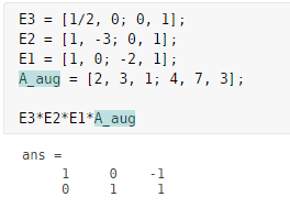
Figure 4. Solution of a system of equations using elementary matrices (MATLAB)