
What KL divergence tells you: The Discrepancy Between Reality and Expectations
prerequisites
In order to understand the contents of this post, it is recommended that you have knowledge of the following:
Cross Entropy
Before delving into the topic of KL divergence, it is necessary to understand the concept of cross entropy, which is essential for understanding KL divergence.
In short, cross entropy can be described as the “surprise (i.e., information) caused by the difference between prediction and reality.”
To understand this concept in more detail, let’s first look at the binary case, where there are only two possible outcomes.
Binary Cross Entropy
In the binary case, there are only two possible outcomes: 0 or 1.
Let’s say we have some data (e.g., height, weight, etc.) and we want to classify it as either “male” or “female.” We can output the result of each classification as 0 or 1.
The cross entropy in the binary case is defined as follows:
If the target is $y$ and the predicted value is $\hat{y}$, then
\[BCE = -y\log(\hat y) - (1-y) \log(1-\hat y)\]where BCE stands for Binary Cross Entropy.
Since the target value and the model output value can both be either 0 or 1, there are four possible cases:
① When $y=1$ and $\hat y = 1$
In this case, the model correctly predicts the target value, and we can see that the BCE value is 0.
\[BCE = -y\log(\hat y) - (1-y) \log(1-\hat y)\notag\] \[=1\cdot \log(1) - 0 \cdot \log(0) = 0\]② When $y=1$ and $\hat{y}=0$,
In this case, the target value was not achieved. We can see that the value of BCE is infinite.
\[BCE = -y\log(\hat y) - (1-y) \log(1-\hat y)\notag\] \[=-1\cdot \log(0) -0\cdot \log(1) = \infty\]③ When $y=0$ and $\hat{y}=1$,
Similar to the previous case, the target value was not achieved, and the value of BCE is also infinite.
\[BCE = -y\log(\hat y) - (1-y) \log(1-\hat y)\notag\] \[=-0\cdot \log(1) - (1)\cdot\log(0) = \infty\]④ When $y=0$ and $\hat{y}=0$,
In the case where the target value is exactly matched, the value of BCE becomes 0.
\[BCE = -y\log(\hat y) - (1-y) \log(1-\hat y)\notag\] \[=-0\cdot\log(0) - (1)\log(1) = 0\]Cross-Entropy with multiple output cases
From the discussion on Binary Cross Entropy, we can understand that Cross Entropy is a measure of how different the target value and the model’s output value are.
In other words, the formula for BCE can also be written like this:
\[BCE = \sum_{x\in{0, 1}}\left(-P(x)\log(Q(x))\right)\]Here, $P(x)$ can be seen as the desired target outcome, and $Q(x)$ can be regarded as the model’s output value.
By generalizing this, we can define Cross Entropy for cases with multiple output possibilities like this:
\[CE = \sum_{x\in\chi}\left(-P(x)\log(Q(x))\right)\]What can we think about from the above Cross Entropy formula?
We can consider CE as a measure of the ‘surprise’ we obtain when we have an ideal value $P$ and observe the results of $Q$ obtained from the model as information.
For example, let’s say we roll a slightly abnormal die as follows:
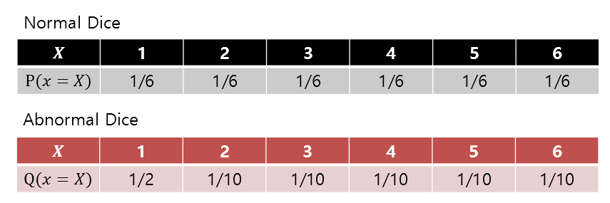
Figure 1. Probability distributions for an ideal (or normal) die and a biased die with more occurrences of 1.
In other words, what this example is discussing is that when we roll a strange die (our model) that is different from an ideal (or normal) die, where the probability of each face is 1/6, we want to know how much ‘surprise’ we get.
If we calculate the Cross Entropy, we get:
\[\Rightarrow -\sum_i P(x_i)\log(Q(x_i)) = -\left(\frac{1}{6} \log_2(1/2) + \frac{5}{6} \log_2(1/10)\right) = 2.9349 \text{ bit}\]On the other hand, if it were an ideal die, the information entropy value would be:
\[\Rightarrow -\sum_i P(x_i)\log(P(x_i)) = -\left(\frac{6}{6}\log_2(1/6)\right) = 2.5850 \text{ bit}\]Therefore, if we expect an ideal die and use the actual value of the die we obtain to calculate the Cross Entropy, we can say that the level of surprise (i.e., the surprise of the discrepancy between the ideal and reality) is greater.
KL divergence: relative comparison of information entropy
KL divergence is short for Kullback-Leibler divergence, where both Kullback and Leibler are confirmed to be human names.
So when thinking about KL divergence, just focus on the word “divergence,” and note that the meaning of this divergence is not like the concept of vector field divergence, but rather simply using another word to mean “difference.”
In particular, the “difference” here refers to comparing two probability distributions.
Since the comparison is made using information entropy, KL divergence is also called relative entropy.
For example, let’s say our goal is to accurately model probability distribution $P$.
If the discrete probability distributions $P$ and $Q$ are defined on the same sample space $\chi$, then KL divergence is as follows:
\[D_{KL}(P\|Q) = \sum_{x\in \chi}P(x)\log_b\left(\frac{P(x)}{Q(x)}\right)\]Here, the base of the logarithm $b$ is usually 2, 10, or $e$, and the unit of information quantity when each is used is bit, dit, or nit, respectively.
Expanding the formula a little more,
\[\Rightarrow-\sum_{x\in \chi}P(x)\log_b\left(\frac{Q(x)}{P(x)}\right)\] \[=-\sum_{x\in\chi}P(x)\log_b Q(x) + \sum_{x\in\chi}P(x)\log_b P(x)\]Looking closely at equation (3), we can see that terms containing two summations can all be thought of as expectations.
\[\Rightarrow -E_P[\log_bQ(x)]+E_P[\log_bP(x)]\]Here, the subscript ‘P’ attached to the expectation operator $E$ means that it is the expectation with respect to the probability distribution $P(x)$.
Expanding formula (4) a little further,
\[\Rightarrow H_P(Q) - H(P)\]where $H_P(Q)$ represents the cross-entropy of $Q$ with respect to $P$ and $H(P)$ represents the information entropy of $P$.
Visualization of KL divergence.
The sum of the areas under the green function with respect to the blue and red functions, denoted as $P(x)$ and $Q(x)$, respectively, represents the value of KL divergence $D_{KL}(P\|Q)$.