The Purpose and Definition of Correlation Coefficient
The correlation coefficient can be used when you want to determine the (correlation) relationship between two variables that change continuously.
For example, you can determine the correlation between weight and height, or between math scores and English scores.
The relationship between two variables that change continuously can also be visually confirmed by creating a scatter plot. By plotting n pairs of values for the two variables on the x-axis and y-axis, you can create a scatter plot.
For example, the scatter plot below shows the math and English scores of 500 students.

Figure 1. Example of a scatter plot. Positive correlation between math scores and English scores is observed.
The correlation coefficient can be defined as follows:
For n datasets,
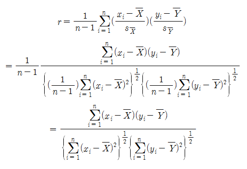
\[r = \frac{1}{n-1}\sum_{i=1}^{n} \left(\frac{x_i-\bar{X}}{s_{\bar{X}}}\right) \left(\frac{y_i-\bar{Y}}{s_{\bar{Y}}}\right)\]If you are asked to determine the correlation for 500 data points, you can simply plug in the numbers into this formula and calculate the result. But what does this formula really mean?
It is related to the concept of inner product of vectors.
Inner Product of Vectors
Let’s consider two arbitrary 2-dimensional vectors $\vec{a}$ and $\vec{b}$.
The inner product of two vectors is defined as follows:
\[\vec{a}\cdot\vec{b} = \sum_{i=1}^{n}a_ib_i\]For example, if we have vectors $\vec{a}=(2,3)$ and $\vec{b}=(3,0)$, the inner product of these two vectors is:
\[\vec{a}\cdot\vec{b} = \sum_{i=1}^{n}a_ib_i = (2\times 3)+(3\times 0) = 6\]
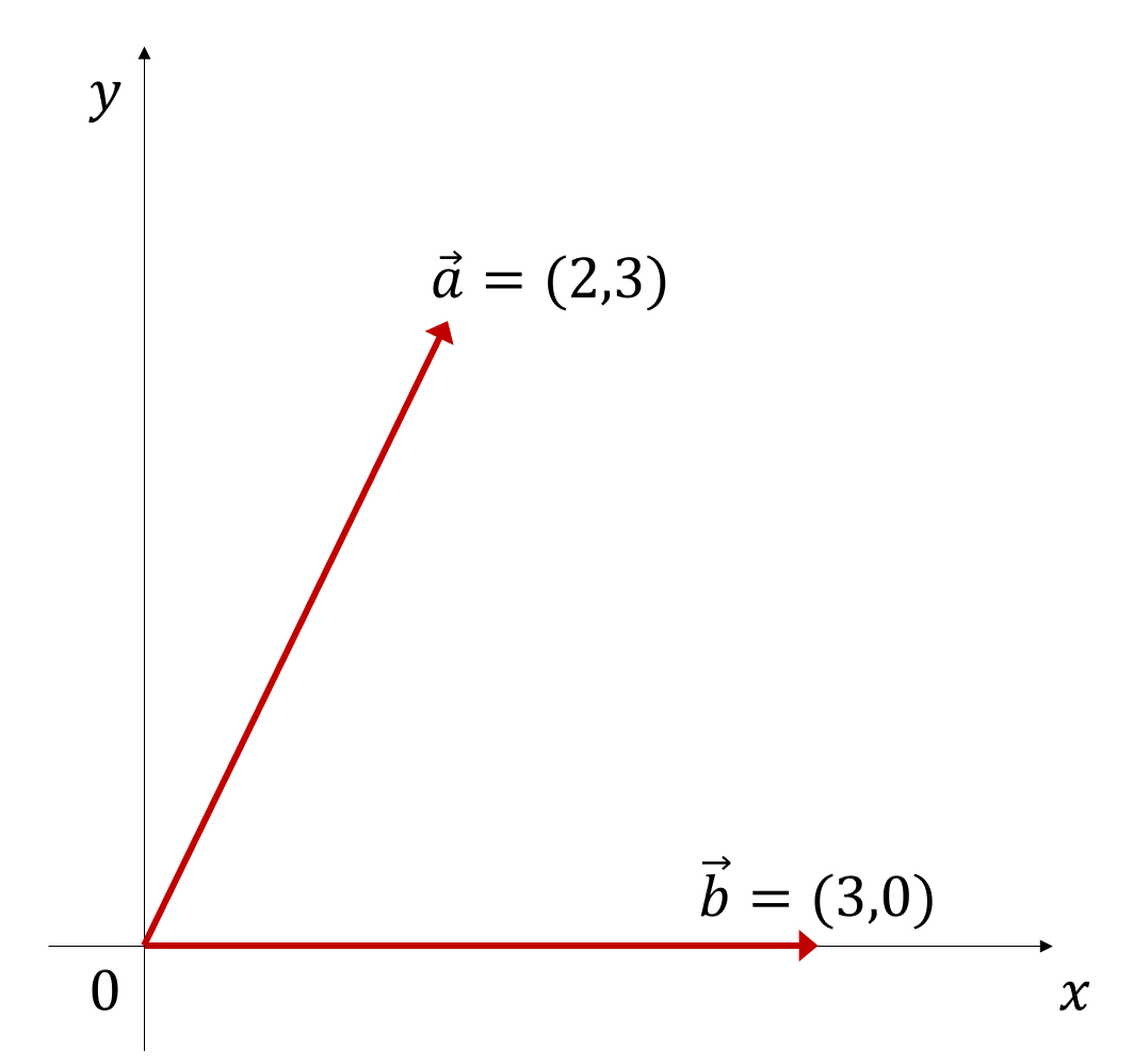
Figure 2. Vectors a = (2,3) and b = (3,0) plotted on a 2D plane.
On the other hand, the dot product of vectors has a geometric interpretation as the product of the length of the projection of vector $\vec{a}$ onto vector $\vec{b}$ and the length of vector $\vec{b}$.
In other words, as shown in Figure 3 below, the dot product of two vectors has the geometric interpretation:
\[\vec{a}\cdot\vec{b} = |\vec{a}|\cos(\theta)\times|\vec{b}|\]This means that the dot product of two vectors can be interpreted as “how much of the change in vector a can be explained by vector b?”
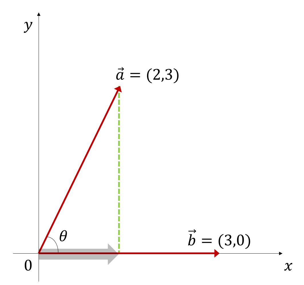
Figure 3. Projection of vector a onto vector b.
Using the dot product of two vectors and the length of vector $\vec{b}$, we can determine the length of the projection of vector $\vec{a}$ onto vector $\vec{b}$.
In other words, the length of the projection of vector $\vec{a}$ onto vector $\vec{b}$, denoted by $proj_b a$, can be calculated as follows:
\[proj_ba = \frac{\vec{a}\cdot\vec{b}}{|\vec{b}|}\]We can also interpret $proj_b a$ in a slightly different way.
Furthermore, it is worth noting that $\vec{a}\cdot\vec{b}=\vec{b}\cdot\vec{a}$, which means that the order of the vectors in the dot product does not matter. Therefore, we can calculate the length of the projection of vector $\vec{b}$ onto vector $\vec{a}$, denoted by $proj_ab$, as follows:
\[proj_ab = \frac{\vec{a}\cdot\vec{b}}{|\vec{a}|}\]Similarly, we can interpret $proj_ab$ as “how much of the change in vector b can be explained by vector a?” as shown in Figure 4 below.
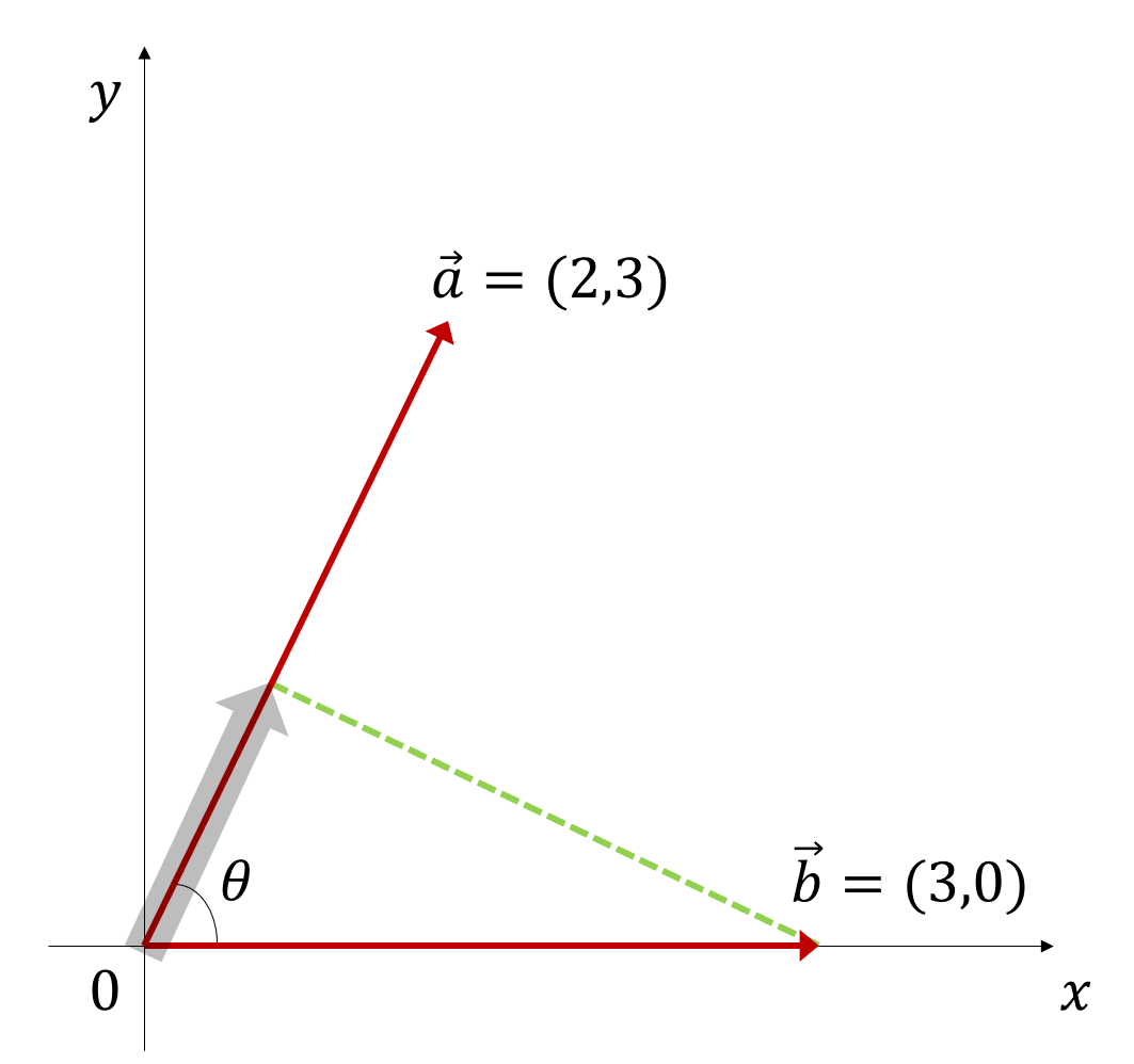
Figure 4. Projection of vector b onto vector a.
In summary, the following explanations can be given:
- To understand the relationship between $\vec{a}$ and $\vec{b}$:
- To grasp the extent to which $\vec{a}$ explains $\vec{b}$:
- To grasp the extent to which $\vec{b}$ explains $\vec{a}$:
Therefore, if $\vec{a}$ and $\vec{b}$ explain each other:
\[\rightarrow \times \frac{1}{|\vec{a}|} \times \frac{1}{|\vec{b}|}\]So, the amount by which $\vec{a}$ and $\vec{b}$ explain each other can be expressed as:
\[\frac{\vec{a}\cdot\vec{b}}{|\vec{a}||\vec{b}|} = \cos(\theta)\]Back to Correlation Coefficient!
Let’s take a look at the formula for the correlation coefficient again:
\[r = \frac{1}{n-1}\sum_{i=1}^{n} \left(\frac{x_i-\bar{X}}{s_{\bar{X}}}\right) \left(\frac{y_i-\bar{Y}}{s_{\bar{Y}}}\right)\]Among these,
\[\frac{x_i-\bar{X}}{s_{\bar{X}}}\]and
\[\frac{y_i-\bar{X}}{s_{\bar{Y}}}\]seem to be closely related to the normalization process. However, this time let’s separate $(x_i-\bar{X})$ and $(y_i-\bar{Y})$, and use the original definitions of $s_{\bar{X}}$ and $s_{\bar{Y}}$ to express $(x_i-\bar{X})$ and $(y_i-\bar{Y})$.
Let’s denote $a_i=x_i-\bar{X}$ and $b_i=y_i-\bar{Y}$.
Then the equation above can be written as follows:
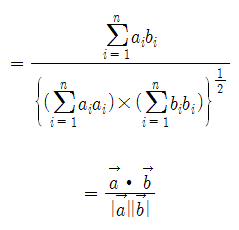
In other words, the correlation coefficient $r$ can be interpreted as:
“How well do $\vec{a}$ and $\vec{b}$ explain each other?”
or
“How well do $x_i-\bar{X}$ and $y_i-\bar{Y}$ explain each other?”
In other words, this means that we are only interested in how much the datasets are spread out from each other, ignoring how far they are from the origin.
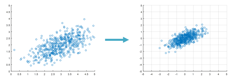
Figure 5. In the left figure, although the center of the scatter plot is (3,2), the correlation is an amount that is independent of how far the dataset is from the origin. Therefore, the equation for correlation allows us to ignore the distance from the origin, as shown in the right figure.
On the other hand,
\[\frac{\vec{a}\cdot\vec{b}}{|\vec{a}||\vec{b}|} = \cos(\theta)\]And,
\[-1\leq\cos(\theta)\leq 1\]So,
\[-1\leq r\leq 1\]This makes it very natural to say that the correlation coefficient $r$ falls between -1 and 1.
The Difference between Correlation Coefficient and Covariance
Both correlation coefficient and covariance can be explained using the inner product of vectors, and they are both connected to the ‘similarity’ between data (i.e., vectors).
However, the most prominent difference between the two is the normalization method. The correlation coefficient normalizes by the magnitude of the vectors, while covariance normalizes by the number of elements in the vectors.