※ To facilitate visualization and understanding, the field (in which vectors and matrices are defined) is limited to real numbers.
Fundamental Matrix Subspaces / Introduction to Linear Algebra(Gilbert Strang, 1993)
Prerequisites
To understand this post, it is recommended that you have knowledge of the following topics:
- Basic operations of vectors (scalar multiplication, addition)
- Another perspective on matrix multiplication
- Matrix and linear transformation
Matrix is a linear transformation
Many discussions related to linear algebra have been constructed based on the fact that “Matrix is a linear transformation.”
To briefly review, a matrix transforms a vector into another vector.
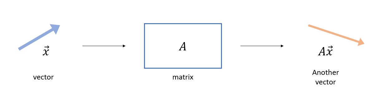
Figure 1. A matrix is an operator that transforms a vector.
In other words, a matrix is a function that takes a vector as input and outputs another vector.
Then, the question we can ask here is whether a linear transformation, if it is a function, can satisfy the fundamental definition of a function.
In other words, just because there are inputs and outputs, can we say that a “linear transformation” is a function?
The most fundamental definition of a function
A function is defined as a mapping between sets.
The rigorous definition of a function is as follows.
| DEFINITION 1. Function |
|---|
| Let $X$ and $Y$ be sets, which are called the domain and the codomain, respectively. Let the graph of $f$ be a subset of the Cartesian product $X \times Y$, and let us call it the graph of $f$. Then, for any $x\in X$, if there exists a unique $y\in Y$ such that $(x,y)\in\text{ graph } f$, we write $f(x)$ for such $y$. |
Since Definition 1 may sound a bit difficult just by reading it, it can be expressed by the following figure.
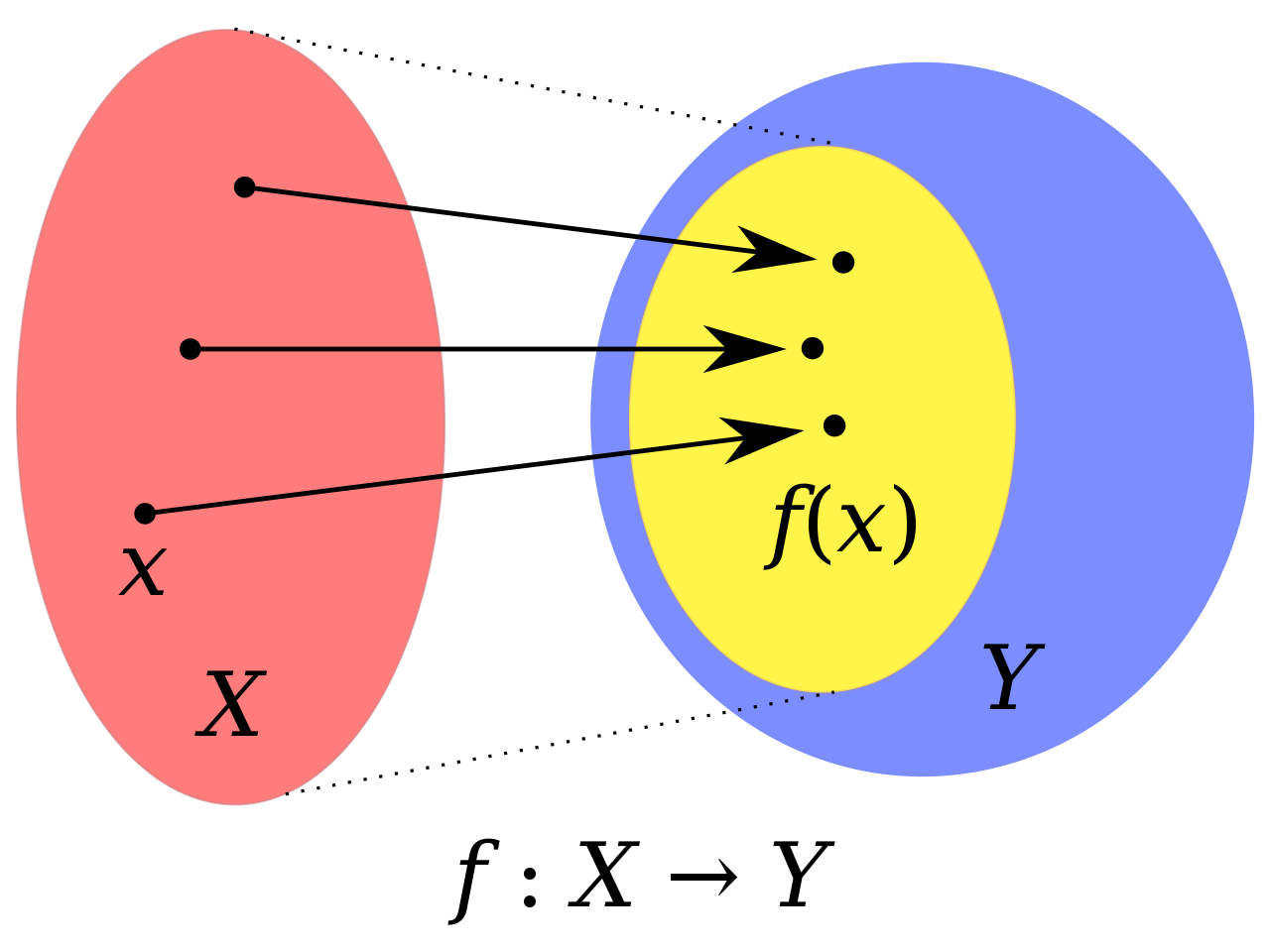
Figure 2. A function maps each element of the domain to exactly one element of the codomain.
Here, $X$, $Y$, and $f(X)$ are the domain, codomain, and range of the function $f$, respectively.
Source: Wikipedia, Function
In Figure 2, the domain $X$, codomain $Y$, and range $f(X)$ of the function $f$ are indicated by red, blue, and yellow, respectively.
In other words, if we think of linear transformations as functions, we should be able to think about the mapping from domain to range, which is the fundamental meaning of a function.
Then, what are the domain, codomain, and range in linear transformations?
That is what the four main subspaces (row space, null space, column space, left null space) mean.
What is a subspace?
A vector space is a set that consists of vectors as its elements.
In a vector space, it is necessary to define two operations (scalar multiplication and addition) in addition to simply collecting elements, which is a slightly expanded concept from the notion of a set.
A subspace can be seen as a concept that applies the notion of a subset to a vector space.
That is, just as there are subsets in sets, there are also small vector spaces, namely subspaces, that maintain the basic structure of the vector space in the vector space.
For example, in a 2-dimensional real space, if we consider a subspace, the set of all vectors on the line passing through the origin forms a 1-dimensional subspace.
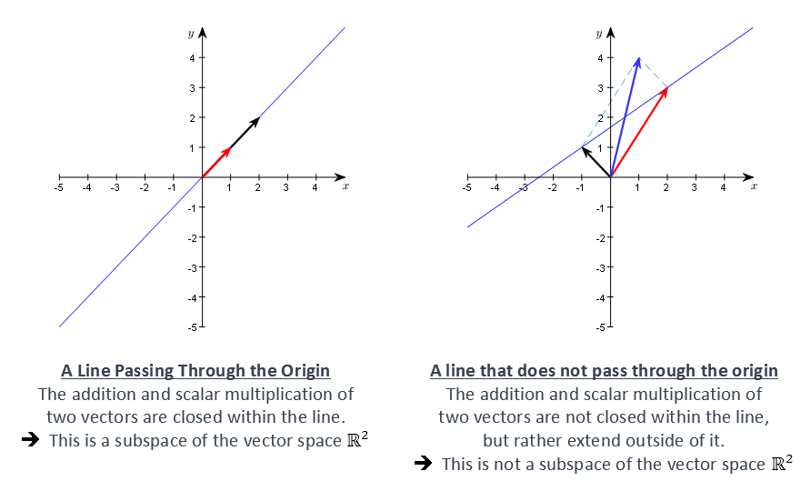
Figure 3. 1-dimensional subspace within the 2-dimensional real space
Row Space and Column Space
From this perspective, the vector space consisting of linear combinations (i.e., span) of all rows or all columns of an arbitrary matrix $A$ given to us is a subspace, and each is called the row space and the column space, respectively.
For example, let’s say matrix $A$ is given as follows.
\[A = \begin{bmatrix}2 && 1 \\ 4 && 2\end{bmatrix}\]Then, the row space is the set of all vectors lying on the line formed by the linear combination of the vectors $\begin{bmatrix} 2 & 1 \end{bmatrix}$ and $\begin{bmatrix} 4 & 2 \end{bmatrix}$.
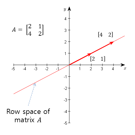
Figure 4. Row space formed by linear combinations of row vectors of matrix A
Also, the column space is the set of all vectors lying on the line formed by the linear combination of the vectors $\begin{bmatrix} 2 & 4 \end{bmatrix}^T$ and $\begin{bmatrix} 1 & 2 \end{bmatrix}^T$.
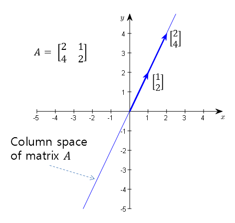
Figure 5. Column space formed by linear combinations of column vectors of matrix A
Null Space
There is also a subspace called the null space that is difficult to immediately recognize in matrix $A$.
The null space is the set of vectors $\vec{x}$ that satisfy the following condition:
\[A\vec{x} = 0\]That is, they are input vectors that make the linear transformation $A$ output 0.
Then, let’s visually consider how the linear transformation $A$ works.
\[A = \begin{bmatrix} 2 & 1 \\ 4 & 2 \end{bmatrix}\]
Animation 1. Linear transformation of matrix A
The noteworthy point in the animation is that all the points (i.e., vectors) that were in the 2D vector space move to the column space after linear transformation.
Let’s compare the column space seen in Figure 5 with the result of linear transformation in the animation.
So, can we capture all the vectors that move to the point (0, 0) after linear transformation?
Most of the points move to the column space, but some points will move to the point (0,0) in the column space.
The set of those points (i.e., vectors) is the null space.
In the animation below, the null space is represented by a yellow line.
Animation 2. Linear transformation of matrix A and null space (yellow line)
An interesting point is that the column space and the null space are orthogonal to each other.
If we display the yellow vector space (i.e., a line passing through the origin) and the column space of matrix A together, as found in the animation above, we can see that they are orthogonal.
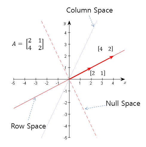
Figure 6. The column space and null space of matrix A are orthogonal to each other
Fundamental theorem of linear algebra
※ What the Fundamental theorem of linear algebra means:
If a matrix is a function, how do we define the relationship between sets, which is the fundamental meaning of the function? ※
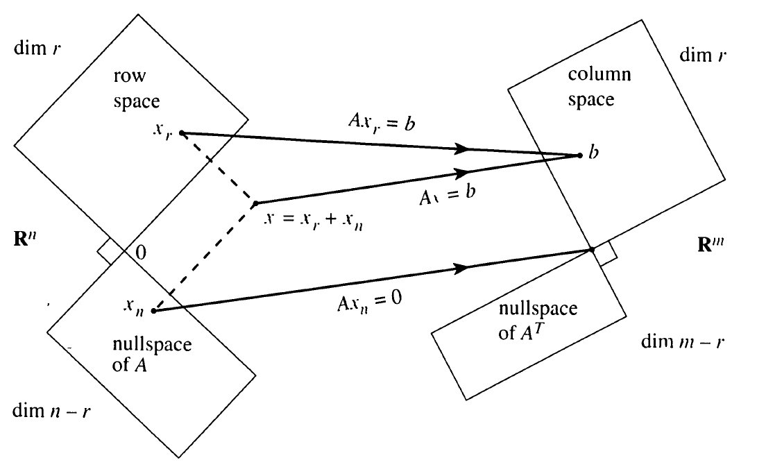
The Fundamental Theorem of Linear Algebra establishes the relationship between the main subspace described in this post, and explains how to view this relationship from the perspective of a function.
More specifically, when viewing the domain and codomain sets as vector spaces, if the matrix has a dimension of $m\times n$, the domain becomes an $n$-dimensional vector space, and the codomain becomes an $m$-dimensional vector space.
In other words, if $A\in \Bbb{R}^{m\times n}$, this matrix can be viewed as a function:
\[f: \Bbb{R}^n \rightarrow \Bbb{R}^m\]Input (Domain): Row Space + Null Space = $\Bbb{R}^n$
The domain of a linear transformation is the union of the row space and the null space.
Any vector in an $n$-dimensional real space can be expressed as a linear combination of vectors in the row and null spaces.
What does this mean? Let’s consider a $2\times 2$ matrix, matrix $A=[2, 1;4, 2]$, that we have dealt with so far.
For example, the vector (2,3) is neither a point (vector) on the row space nor a point (vector) on the null space.
However, by using the fact that the row space and the null space are orthogonal to each other, the vector (2,3) can be expressed as a linear combination of the bases of the row and null spaces.

Figure 7. Any vector in the domain can be expressed using both the row space and the null space.
Output (Range): Everything is in the Column Space
As seen in Animation 2, all vectors in the domain are transformed into points on the column space.
This is because, as seen in Another Perspective on Matrix Multiplication, the product of a matrix and a vector can be expressed as a linear combination of column vectors.
Another interpretation is that all vectors in the domain are composed of linear combinations of the bases of the row space and null space, and the elements of the vectors expressed by the null space bases decrease in size to 0 after the linear transformation. Therefore, after the linear transformation, all vectors are positioned on the column space.
Codomain: $m$-dimensional Real Space
The codomain of a linear transformation is the column space. The left null space is obtained by subtracting the column space from the codomain.
In a linear transformation function, the codomain is the sum of the column space and the left null space, and the column space and left null space are orthogonal to each other.
The left null space cannot be visualized in the linear transformation process, but it can be expressed as follows because it is orthogonal to the column space.
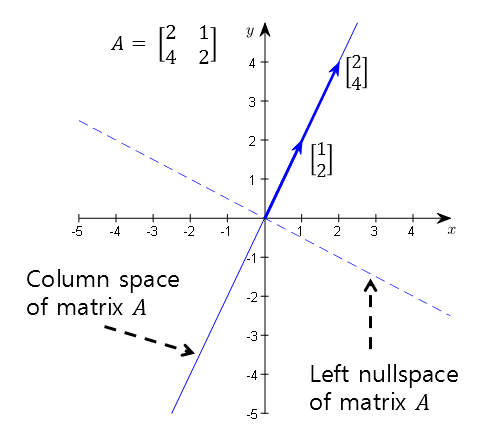
Figure 8. The codomain consists of the column space and left null space, and the two subspaces are orthogonal to each other.