This post is written with reference to Professor Nathan Kutz’s lecture.

Prerequisites

To understand this post well, it is recommended that you know about the following:

• Eigenvalues and eigenvectors
• Linear operators and function spaces

Introduction to Hermitian matrices

A Hermitian matrix is a complex square matrix whose transpose is equal to its conjugate. In other words, for any $n\times n$ matrix, if the following property holds, it is a Hermitian matrix:

\[A^H=A\]

That is,

\[A_{ij}=\bar{A_{ji}}\]

Here, $A^H$ denotes the conjugate transpose, and $\bar{A}$ denotes the complex conjugate.

Hermitian matrices extend the concept of transpose matrices used in real matrices to the complex system.

For example, the following matrices are Hermitian matrices:

\[\begin{bmatrix} 2 & 2+i & 4 \\ 2-i & 3 & i \\ 4 & -i & 1\end{bmatrix}\]

Key properties

Some important properties of Hermitian matrices are listed below.

1. The diagonal elements of a Hermitian matrix are always real.

Proof:

Suppose $A$ is an $n\times n$ Hermitian matrix. Then, for $i=1, 2, \cdots, n$, we have:

\[A_{ii}=\bar{A_{ii}}\]

Thus, the imaginary part of $A_{ii}$ is 0.

2. The eigenvalues of a Hermitian matrix are always real numbers.

Proof:

Let $\lambda \in \Bbb{C}$ be an eigenvalue of the Hermitian matrix $A$. Then, there exists an eigenvector $v\neq 0$ such that

\[Av=\lambda v\]

Now, let’s take the inner product of $Av$ and $v$. We can express inner product as $\langle \cdot, \cdot \rangle$. Then,

\[\langle Av, v\rangle=(Av)^Hv=v^HA^Hv=\langle v, A^Hv\rangle=\langle v, Av \rangle\]

We know that $Av=\lambda v$ by the definition of eigenvalue and eigenvector. Therefore, the leftmost equation in the above equation becomes

\[\langle Av, v\rangle = \langle \lambda v, v\rangle=\bar \lambda v^Hv\]

On the other hand, the rightmost equation in the above equation becomes

\[\langle v, Av\rangle=v^H\lambda v=\lambda v^Hv\]

Since the eigenvector is not the zero vector, $v^Hv$ is not zero.

Therefore,

\[\lambda = \bar\lambda\]

Thus, the eigenvalue $\lambda$ is always a real number.

3. The eigenvectors corresponding to different eigenvalues of a Hermitian matrix are orthogonal to each other.

Proof:

Let $v_1$ and $v_2$ be nonzero $n$-dimensional complex vectors in $\Bbb{C}^n$, which are the eigenvectors of the matrix $A$ corresponding to different eigenvalues $\lambda_1\neq \lambda_2$. Now, let’s take the inner product of $Av_1$ and $v_2$. Then,

\[\langle Av_1, v_2\rangle=(Av_1)^Hv_2=v_1^HA^Hv_2=\langle v_1, A^Hv_2\rangle=\langle v_1, Av_2\rangle\]

We can express inner product as $\langle \cdot, \cdot \rangle$. The leftmost equation in the above equation becomes

\[\langle Av_1, v_2\rangle = \langle \lambda_1v_1, v_2\rangle=\lambda_1\langle v_1, v_2\rangle\]

and the rightmost equation becomes

\[\langle v_1, Av_2\rangle=\langle v_1, \lambda_2 v_2\rangle=\lambda\langle v_1, v_2\rangle\]

The two equations are identical, so

\[\lambda_1\langle v_1, v_2\rangle = \lambda_2\langle v_1, v_2\rangle\] \[\Rightarrow (\lambda_1-\lambda_2)\langle v_1, v_2\rangle = 0\]

Here, since $\lambda_1 \neq \lambda_2$, $\langle v_1, v_2\rangle = 0$.

Therefore, two eigenvectors corresponding to different eigenvalues are orthogonal to each other.

(P.S.)¹

What if the two eigenvalues of a Hermitian matrix are the same?

One of the Hermitian matrices with two equal eigenvalues is the unit matrix.

For example, considering the following matrix,

\[\begin{bmatrix}1 & 0\\0 & 1\end{bmatrix}\]

Both eigenvalues are 1, and any vector direction can be an eigenvector. This can be generalized as follows:

If two eigenvalues are equal, then two linearly independent vectors $v_1$ and $v_2$ can be chosen within the vector space generated by these two vectors.

In other words, for any matrix $A$,

\[A(av_1+bv_2)=a Av_1+bAv_2 = a\lambda v_1 + b\lambda v_2 = \lambda(av_1 + bv_2)\]

Therefore, it is possible to select any two vectors within the vector space spanned by $v_1$ and $v_2$, and they do not have to be orthogonal, but it is possible to select two orthogonal vectors.

Representation of solution using eigenvectors

Let $A$ be an $n\times n$ Hermitian matrix,

\[Ax_i=\lambda_i x_i \quad\text{ for }\quad i=1,2,\cdots,n\]

consider $n$ eigenvalues $\lambda_i$ and eigenvectors $x_i$ such that they are orthogonal if the eigenvalues are distinct.

Therefore, any vector in the $n$-dimensional complex space can be expressed as a linear combination of eigenvectors.

Thus, when solving the $Ax=b$ problem, the solution $x$ can also be expressed as follows.

\[x=\sum_{i=1}^{n}c_i x_i\]

That is, we can represent the solution $x$ using eigenvectors, and what we need to know is the value of $c_i$ regarding how much we will use the basis vectors.

Since we know both the eigenvector $x_i$ and the $b$ vector for $Ax=b$, we can obtain the value of $c_i$ as follows.

For the equation,

\[Ax=b\]

we can express $x$ using eigenvectors as follows.

\[A\sum_{i=1}^n c_ix_i=b\]

Let’s take the inner product of both sides with the eigenvector $x_j$.

\[A\sum_{i=1}^n c_ix_i\cdot x_j=b\cdot x_j\]

By placing $A$ inside the summation, we can rewrite the equation as follows, using the definitions of eigenvalues and eigenvectors.

\[\Rightarrow \sum_{i=1}^n c_i\lambda_i x_i\cdot x_j=b\cdot x_j\]

If $A$ is a Hermitian matrix and all the eigenvalues are distinct, different eigenvectors are orthogonal to each other. Therefore, $x_i\cdot x_j$ in the above equation is only 1 if $i=j$ and 0 otherwise. Hence,

\[\Rightarrow c_j\lambda_j (x_j\cdot x_j) = b\cdot x_j\] \[=c_j\lambda_j=b\cdot x_j\]

Therefore, $c_i$ can be calculated as follows:

\[c_i = \frac{b\cdot x_i}{\lambda_i}\]

Therefore, the solution to the $Ax=b$ problem can be expressed using eigenvectors and eigenvalues as follows:

\[x=\sum_{i=1}^{n}c_ix_i=\sum_{i=1}^{n}\left(\frac{b\cdot x_i}{\lambda_i}\right)x_i\]

The interesting point is that with this method, the solution can be obtained without necessarily calculating the inverse.

Expansion of Eigenfunctions

Introduction to the Concepts of Eigenvalues and Eigenfunctions

When solving the $Ax=b$ problem in linear algebra, the solution $x$ can be obtained by expressing it as a linear combination of eigenvectors. Similarly, in functional analysis, the solution function $u$ of the $Lu=f$ problem can also be obtained by expressing it as a linear combination of eigenfunctions.

Let’s consider the concepts of eigenvalues $\lambda_n$ and eigenfunctions $u_n$ for a linear operator $L$.

As we saw in the previous Linear Operator and Function Space post, just as a matrix acts as a function that takes in a vector and outputs a vector,

we can also consider a new type of function that takes in a function and outputs a new function. The linear operator is the tool that relates these input-output functions.

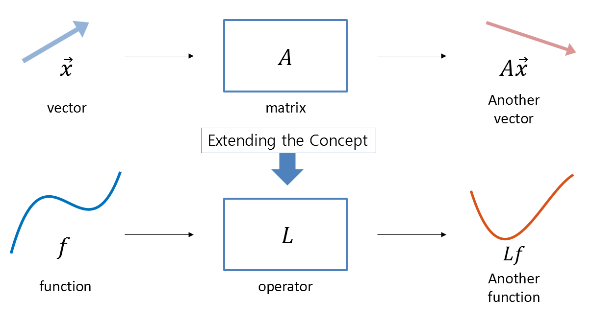
Figure 1. The relationship between vectors and matrices extends to the relationship between functions and operators.

On the other hand, in linear algebra, we defined eigenvalues and eigenvectors. This concept says that if we can find a vector such that the vector outputted by applying the matrix to that vector is only a scalar multiple of the input vector, then that vector is an eigenvector and the scalar multiple is the eigenvalue.

This concept can be extended to linear operators, which also have the concepts of eigenvalues and eigenfunctions.

In other words, we can come up with functions $u_n$ and $\lambda_n$ that satisfy the following relationship:

\[Lu_n=\lambda_n u_n \quad\text{for}\quad n = 1, 2, \cdots, \infty\]

What this equation tells us is that when the linear operator $L$ is applied to the function $u_n$, the function $u_n$ is only scaled by the constant $\lambda_n$ of the input function.

Expansion using orthogonal eigenfunctions

As we were able to express the solution using the linear combination of eigenvectors in the early part of this post, we can also express the solution of $Lu=f$ using the linear combination of eigenfunctions.

Let’s consider the following differential equation:

\[Lu=f\]

Assume that the operator $L$ has an infinite number of orthogonal eigenfunctions $u_n \quad\text{for}\quad n = 1, 2, \cdots \infty$ ². Also, assume that the norms of these eigenfunctions are all 1.

Then, the solution function $u$ of $Lu=f$ can be expressed using the eigenfunctions $u_n$ as a new basis as follows:

\[u(x)=\sum_{n=1}^{\infty}c_n u_n\]

This is called the eigenfunction expansion.

On the other hand, let’s define the inner product operation between two functions defined on the interval $[a,b]$ as follows:

\[\langle f, g\rangle=\int_{a}^{b}f^*(x)g(x) dx\]

Here, $^*$ denotes the complex conjugate.

And the norm of a function is defined as follows using the inner product:

\[\text{norm}(f)=\sqrt{\langle f,f\rangle}\]

Now let’s try to solve the equation $Lu=f$ using the eigenfunctions as follows.

\[Lu=L\sum_{n=1}^{\infty}c_nu_n=f\]

Then, by taking the inner product of both sides with eigenfunction $u_m$, we get:

\[\Rightarrow \langle L\sum_{n=1}^{\infty}c_n u_n, u_m\rangle=\langle f, u_m\rangle\]

Since the operator $L$ is a linear operator, we can put $L$ inside the summation as follows:

\[\Rightarrow \langle \sum_{n=1}^{\infty}c_nLu_n, u_m \rangle = \langle f, u_m \rangle\]

By the definition of eigenvalues and eigenfunctions, we can rewrite the equation as follows:

\[\Rightarrow \langle\sum_{n=1}^{\infty}c_n\lambda_n u_n, u_m\rangle=\langle f,u_m\rangle\]

Here, since all different eigenfunctions are orthogonal to each other, $\langle u_n, u_m\rangle$ is only 1 when $u_n$ and $u_m$ are the same, and all other values are 0. Therefore,

\[\Rightarrow c_m\lambda_m=\langle f, u_m\rangle\]

Thus, we can say that we have found the coefficients $c_n$ necessary to expand $u(x)$ into eigenfunctions. Therefore, the expansion of $u(x)$ into eigenfunctions is as follows:

\[u(x)=\sum_{n=1}^{\infty}c_n u_n=\sum_{n=1}^{\infty}\frac{\langle f,u_n\rangle}{\lambda_n}u_n\]

Example Problem

Let’s perform an eigenfunction expansion for the following boundary value problem:

\[-\frac{d^2}{dx^2}u(x)=f(x)\quad u(0)=0, u(l)=0\]

Solution

If we consider the above problem as a problem of $Lu=f$, we can see that the operator $L$ is

\[L=-\frac{d^2}{dx^2}\]

Therefore, let’s consider the following equation to solve the eigenvalue problem for this operator:

\[Lu=\lambda u\] \[\Rightarrow -\frac{d^2}{dx^2}u=\lambda u\] \[\Rightarrow \frac{d^2}{dx^2}u+\lambda u = 0\]

This equation is a general second-order homogeneous differential equation, and its solution is

\[u=c_1\sin{\sqrt{\lambda}}x+c_2\cos{\sqrt{\lambda}}x\]

Now, applying the boundary conditions, we have

\[u(0) = c_2\cos(0)=0\] \[\therefore c_2 = 0\] \[u(l)=c_1\sin\sqrt{\lambda}x=0\]

Here, the important part is that if we make $c_1$ 0, the solution becomes $u(x)=0$, resulting in a trivial solution. Therefore, we can see that we need to set the eigenvalue as follows to avoid getting a trivial solution.

\[\sqrt\lambda =\frac{n\pi}{l}\]

Therefore, the eigenfunctions are given by

\[u_n=\left\lbrace\sin\frac{n\pi x}{l}\right\rbrace\quad\text{for }n\in\Bbb{N}\]

However, since the norms of these eigenfunctions are not 1, let’s normalize them so that they become eigenvectors with a size of 1.

The size of each eigenfunction is

\[\sqrt{\int_{0}^{l}\sin\left(\frac{n\pi x}{l}\right)\sin\left(\frac{n\pi x}{l}\right)dx}=\sqrt{\frac{l}{2}}\]

Therefore, the normalized eigenfunctions are

\[u_n=\left\lbrace\sqrt{\frac{2}{l}}\sin\frac{n\pi x}{l}\right\rbrace\quad\text{for }n\in\Bbb{N}\]

These eigenfunctions can be easily shown to be orthogonal using the inner product of functions.

\[\langle u_n, u_m\rangle=\int_{0}^{l}\left(\sqrt{\frac{2}{l}}\sin\frac{n\pi x}{l}\right)\left(\sqrt{\frac{2}{l}}\sin\frac{m\pi x}{l}\right)dx\] \[=\int_{0}^{l}\frac{l}{2}\sin\left(\frac{n\pi x}{l}\right)\sin\left(\frac{m\pi x}{l}\right)dx\] \[=\begin{cases}0 & m\neq n\\ 1 &m=n\end{cases}\]

Therefore, the solution $u(x)$ that satisfies the original problem can be expressed as a sum of the eigenfunctions with coefficients determined by the inner product.

\[u(x)=\sum_{n=1}^{\infty}c_n\sqrt\frac{2}{l}\sin\left(\frac{n\pi x}{l}\right)\] \[c_n = \frac{\langle f, u_n\rangle}{\lambda_n}\]

If we assume that $f(x) = x$ and $l=1$, then

\[c_n =\frac{1}{(n\pi)^2}\int_{0}^{1}(x)\sqrt{2}\sin\left(n\pi x\right)dx\] \[=\frac{\sqrt{2}}{n^2\pi^2}\int_{0}^{1}x\sin(n\pi x)dx\]

This can be written using integration by parts as follows.

\[\Rightarrow \frac{\sqrt{2}}{n^2\pi^2}\left(x\cdot\frac{-1}{n\pi}\cos(n\pi x)\right)\Big|_{0}^{1}-\int_{0}^{1}\left(\frac{-1}{n\pi}\right)\cos(n\pi x)dx\] \[=\frac{\sqrt{2}}{n^2\pi^2}\cdot\left(\frac{-1}{n\pi}\right)\cos(n\pi)\] \[=(-\sqrt{2})\frac{(-1)^n}{n^3\pi^3}\]

and this leads to the following.

\[u(x) = \sum_{n=1}^{\infty}c_n\sqrt\frac{2}{l}\sin\left(\frac{n\pi x}{l}\right)=\sum_{n=1}^{\infty}(-\sqrt{2})\frac{(-1)^n}{n^3\pi^3}\sqrt{2}\sin(n\pi x)\]

Rewriting the differential equation,

\[-\frac{d^2u}{dx^2}=x\]

with boundary conditions $u(0)=0$ and $u(1)=0$. It can be easily verified that the solution to this equation is

\[u(x) = \frac{x(1-x^2)}{6}\]

Using the eigenfunction expansion method, the solution can be approximated by gradually adding up the solution expressions for each eigenfunction from $n=1$.