Starting…

In daily life, there are times when we give and receive signals. We stop and start again at traffic lights while driving. We call a dog with a gesture, or we urge a friend who is walking towards us from a distance with body language.

So, when we think about it, the word ‘signal’ is widely used in everyday life. If we abstractly define the concept of a signal used in everyday life, it seems to be related to conveying information.

What about systems? The term ‘system’ seems to be a bit more formal and is not directly used in everyday life.

The word ‘system’ is used in terms like ‘social safety net system,’ and the term ‘operating system’ is used to refer to Windows or Mac OS.

When we say ‘system,’ it feels systematic, and it seems to refer to a collection of concepts as a whole.

Before embarking on a series of studies in signal processing, we want to define signals and systems simply. And we will encounter signals/systems with quite different meanings than the terms ‘signal’ and ‘system’ we usually think of.

The first obstacle when studying a new subject is vocabulary. However, if you can accept new terms well, it can be a useful stepping stone for you to see the big picture of the subject.

Signals and Systems

What is a Signal?

There could be various definitions of signals, but it would be good to define the signal we want to study as a pattern of changes to represent information.

Here, ‘change’ refers to changes in time or space.

A signal that shows a pattern of changes over time is also called a time-series or a time signal. In a way, the term ‘pattern’ here has a similar meaning to ‘function.’

And mathematically, signals can be represented using functions. From the perspective that a signal is a function of time, we can express a signal as $s(t)$.

For example, we can consider a voice signal that has been micro-recorded, denoted as $v(t)$, as a function of time on the $x$-axis and as a function of microphone time on the $y$-axis.

Figure 1. Voice signal recorded from a bell

---

Meanwhile, time signals can be broadly divided into two types: continuous-time signals and discrete-time signals¹.

The commonly known analog signal is a continuous-time signal. Mathematically, a continuous-time signal can be represented by a real function. This means that the $x$-axis is the real number line.

The voice signal from the microphone mentioned as an example may be a continuous-time signal.

Discrete signals may be unfamiliar to some. A signal obtained by sampling a continuous-time signal is a discrete signal. We will learn more about sampling later, but it can be described as the process of obtaining values at intermediate points in time when a continuous-time signal changes over time. Therefore, in mathematical terms, a discrete signal is closer to a sequence than a function.

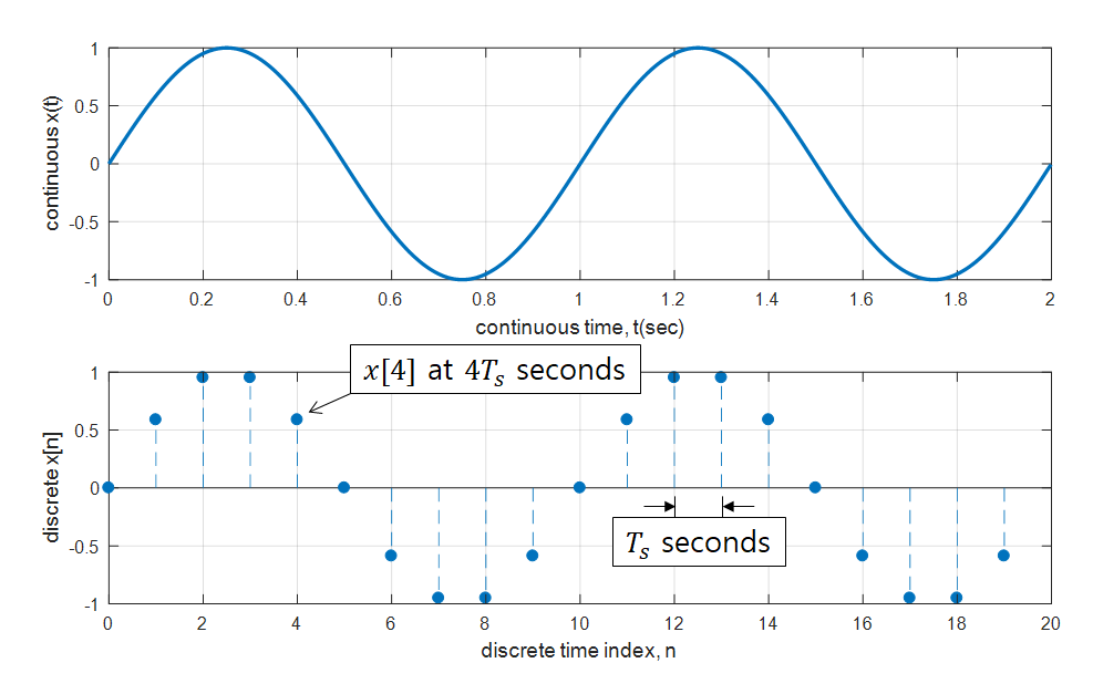
Figure 2. An example of sampling a continuous signal into a discrete signal

The $x$-axis of a discrete signal is denoted as $n$ instead of time $t$, where $n$ is an integer and takes on values such as $\lbrace \cdots, -1, 0, 1, 2, \cdots \rbrace$.

When expressing a discrete signal as a function, square brackets [] are used instead of parentheses ().

Thus, continuous-time signals can be written as $s(t)$, while discrete signals can be written as $s[n]$.

Although it may seem like all signals can be represented using continuous-time signals, the reason why we need to learn about discrete signals is that digital devices cannot represent the concepts of ‘continuous’ and ‘infinite’. Since digital devices cannot represent continuous time, all signals are represented and analyzed using sequences arranged discretely.

---

On the other hand, there are signals that show patterns that change in space, not time. We often refer to these signals as images.

These signals can also be seen as functions composed of two independent variables, such as $p(x,y)$.

Here, $p(x_0, y_0)$ represents the brightness at the position $(x_0, y_0)$.

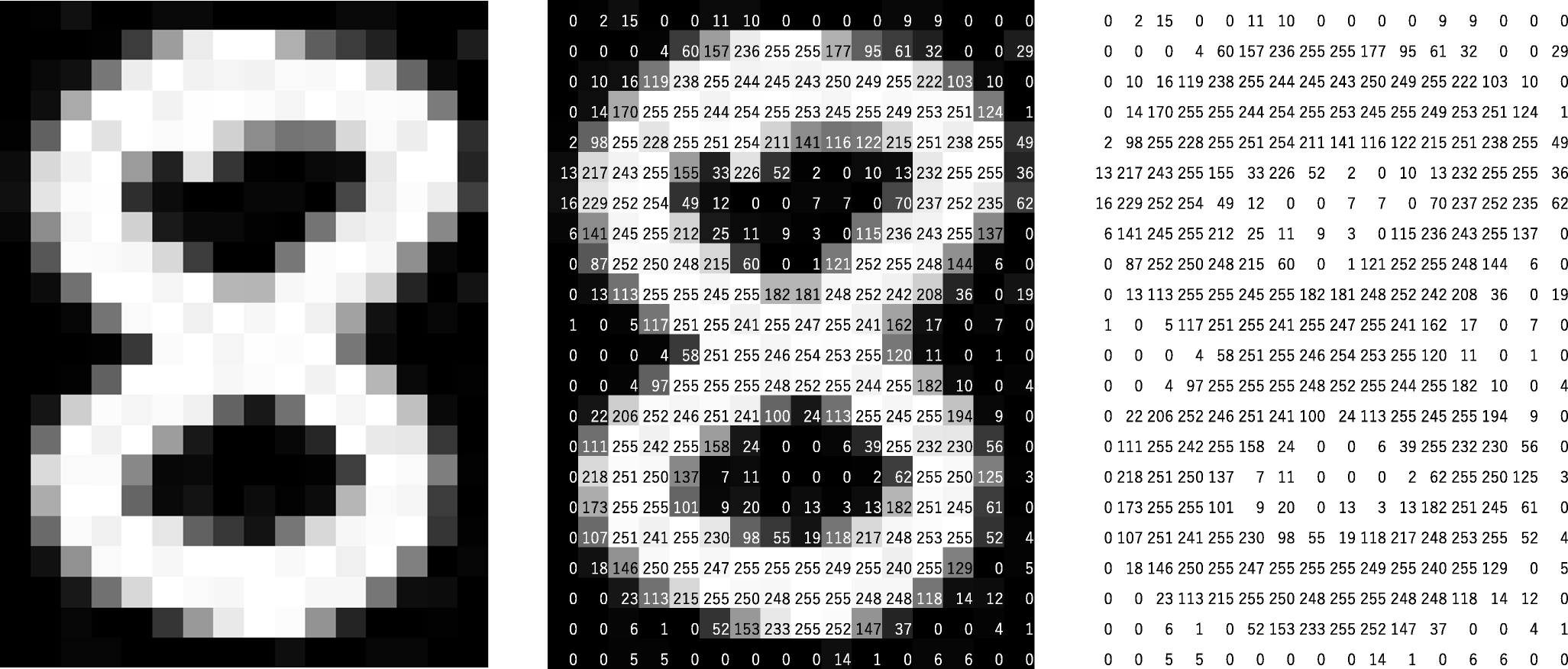
Figure 3. An image can be processed by replacing the brightness of the black and white pixels with numbers ranging from 0 to 255.
Source: Mozanunal.com

Similarly to images, when expressing them using digital devices, they are discretized. Each point on the discretized image is also called a pixel.

Although we mentioned patterns that change in space, in future posts, we will mainly discuss signals in terms of time. (If the opportunity arises, let’s also study images, which are spatial signals, in image processing.)

What is a System?

Unlike various other ‘systems’ mentioned at the beginning of the article, the system discussed in signal processing refers to a function that transforms a signal into a new signal or a different signal representation.

In other words, it can be seen as a concept that is responsible for the transformation between input and output signals.

In signal processing, the input signal is usually denoted as $x(t)$ and the output signal as $y(t)$.

From the perspective of transformation, if the system is represented as $T$, the relationship between input and output can be expressed as follows:

\[y(t)=T\lbrace x(t) \rbrace\]

For example, the input-output relationship of a system that doubles the input signal is as follows:

\[y(t) = 2 x(t)\]

Or the input-output relationship of a system that differentiates the input signal is as follows:

\[y(t) = \frac{d}{dt}x(t)\]

The type of system is distinguished according to the type of input and output.

• If both input and output are continuous-time signals, it is called a continuous-time system.

• If both input and output are discrete signals, it is called a discrete-time system.

• In some cases, there may be a system that receives continuous-time signals as input and discrete signals as output. Analog-Digital Converter can be classified as such a system.

• Also, there may be a system that receives discrete signals as input and continuous-time signals as output. Digital-Analog Converter can be classified as such a system.

Meanwhile, if signals are represented as graphs on the $x$ and $y$ axes, the visual representation of a system is expressed using a block diagram.

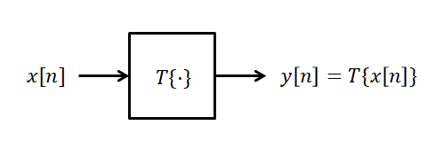
Figure 4. The system can be represented by a block diagram, which connects the input and output.

Connection to Linear Algebra

※ You can understand this section better if you know the following information.

• Basic Operations of Vectors (Scalar Multiplication, Addition)

Signals and systems can be related to the concepts of vectors and matrices in linear algebra.

Since considering signals as a sequence of numbers does not violate the definition of a vector, signals are often represented as a column vector in digital devices.

In other words, if we consider a discrete signal $x[k]$ defined for $k=0, 1, \cdots, n-1$, we can represent it as a column vector like below².

\[x[k]=\begin{bmatrix}x[0] \\ x[1] \\ \vdots \\ x[n-1] \end{bmatrix}\]

Moreover, a system can be represented as a matrix from the perspective that the function of a matrix is a linear transformation between input and output vectors.

However, in this case, the system should be a discrete system that deals with finite-length discrete signals and should be limited to linear systems.

Not all linear discrete systems can be represented as matrices.

For example, the following system is a linear system:

\[y[n]=x[n]-x[n-1]\]

If we limit the length of the signal to $0~(n-1)$ and expand the expression, we get the following:

\[\begin{matrix}y[0] = x[0] \\ y[1]=x[1]-x[0] \\ y[2] = x[2] - x[1] \\ \vdots \\ y[n-1] =x[n-1]-x[n-2]\end{matrix}\]

Therefore, if we represent this system as a matrix, it will be as follows:

\[\begin{bmatrix}y[0] \\ y[1] \\ \vdots \\ y[n-1]\end{bmatrix}= \begin{bmatrix} +1 & 0 & 0 & \cdots & 0 & 0 \\ -1 & +1 & 0 & \cdots & 0 & 0 \\ 0 & -1 & +1 & \cdots & 0 & 0 \\ \vdots & \vdots & \vdots & \cdots & \ddots & \vdots \\ 0 & 0 & 0 & \cdots & -1 & +1 \end{bmatrix} \begin{bmatrix}x[0]\\x[1]\\\vdots \\x[n-1]\end{bmatrix}\]

On the other hand, systems like the following are not linear systems and cannot be represented by matrices:

\[y[n]=(x[n])^2\]

If a discrete system can be represented by a matrix, various skills used in linear algebra can be applied, allowing for analysis of the system from multiple perspectives.

For example, the discrete Fourier transform can be calculated by constructing a Fourier matrix, which is a representative example.