이 문서의 한국어 버전은 아래의 위치에서 찾을 수 있습니다. (You can find a Korean version of this article as below.)
The derivation process of DTFS can be considered very similar to the derivation process of CTFS. The concept of decomposing a periodic function using the orthogonality of trigonometric functions is used identically.
Prerequisites
To understand this post well, it is recommended to have knowledge of the following topics:
Frequency Characteristics of Discrete Sinusoidal Signals
A discrete signal is obtained by sampling a continuous signal in time. At first glance, it may seem that by making the sampling period very short, the discrete signal would look similar to a continuous signal, and thus the analysis can be performed without much difference from continuous signals.
However, through the sampling process, discrete sinusoidal signals exhibit unique frequency characteristics as an additional effect.
In the discrete-time Fourier series, just like in the continuous-time Fourier series, we analyze periodic signals using complex sinusoidals.
Therefore, let’s consider the sampled complex sinusoidals.
For example, a complex sinusoidal with a period of 6 can be expressed as follows:
\[\exp\left(j\frac{2\pi n}{6}\right)\text{ where } n\in \mathbb{N}\]If we plot the points on the complex plane by substituting values for $n$ starting from 0, we can observe the following results:
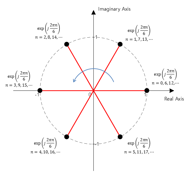
Figure 1. Complex sinusoidal with a Period of 6
In other words, the values of a complex sinusoidal with a period of 6 correspond to 6 points on the unit circle divided into six equal parts on the complex plane.
And the 6 points on the unit circle exhibit periodicity of $2\pi$ due to the nature of the circle. In other words, even the point (1,0) on the complex plane could be a point that has traveled around the circle once or twice.
Therefore, in discrete signals, we can observe that discrete sinusoidals with frequencies that differ by multiples of $2\pi$ or integers of 1 are the same signals. From another perspective, the frequency spectrum of a discrete signal is a periodic function with a period of $2\pi$ or a digital frequency of 1.
The below figure compares the spectrum of a periodic signal with the result of discretizing it through time sampling.
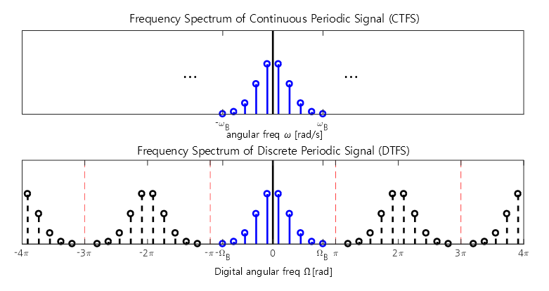
Figure 2. The frequency spectrum of a discrete periodic signal is displayed with copies of the original continuous periodic signal spaced at intervals of $2\pi$.
Furthermore, the following figure compares the spectrum of a non-periodic signal with the result obtained by sampling and discretizing it in time.
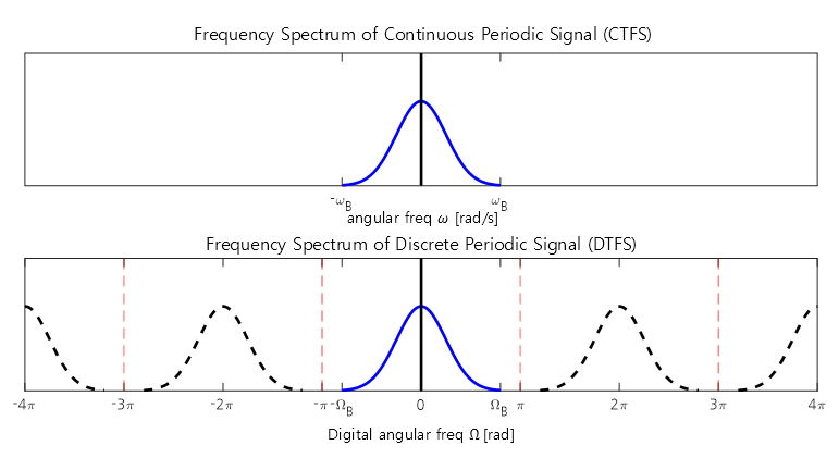
Figure 3. The frequency spectrum of a discrete non-periodic signal is displayed with copies of the original continuous signal spaced at intervals of $2\pi$.
Discrete Time Fourier Series
Discrete Time Fourier Series (DTFS) is a Fourier analysis method that can be applied to periodic discrete signals.
A periodic discrete signal refers to a discrete signal that satisfies $x[n+N] = x[n]$ for an integer period $N$.
For example, the signal shown below can be considered as a periodic discrete signal with a period of 6.
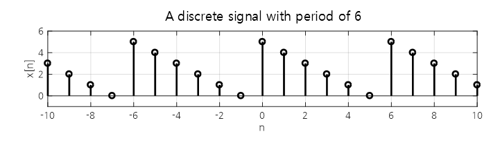
Figure 4. Periodic discrete signal with a period of 6
DTFS is similar to Fourier Series in that it represents the original signal as a linear combination of sinusoidals, with the use of complex sinusoidals being common.
(Refer to the part on Signal Space for the reason why complex sinusoidals are used)
If the period of the discrete signal we want to analyze is $N$, then the fundamental frequency of this signal is $1/N$, and the frequency of the $k$-th harmonic is $k/N$, as easily seen from the “$2\pi$ periodicity” mentioned earlier. By this periodicity, the sinusoidals of $k$ and $k+N$, $k+2N$, $\cdots$ cannot be distinguished from each other. In other words,
\[\exp\left(j\frac{2\pi}{N}(k+mN)n\right)=\exp\left(j\frac{2\pi}{N}kn\right)\exp\left(j2\pi m n\right)=\exp\left(j\frac{2\pi}{N}kn\right)\]holds.
Therefore, for a periodic discrete signal, the number of distinct frequency components cannot exceed $N$.
Hence, the original periodic signal $x[n]$ can be represented as a linear combination of a total of $N$ discrete complex sinusoidals.
\[x[n]=\sum_{k=0}^{N-1}a_k\exp\left(j\frac{2\pi k}{N}n\right)\]Orthogonality of Discrete Complex Harmonic Signals
As we confirmed in the Fourier series, complex harmonic signals with different frequencies are orthogonal to each other.
Two discrete signals $\phi_k[n]$ and $\phi_p[n]$ are said to be orthogonal with respect to period N if the following holds:
\[\sum_{n=0}^{N-1}{\phi_k[n]\phi^*_p[n]} = 0 \text{ when } k\neq p\]Here, ‘*’ in $\phi^*_p[n]$ denotes the complex conjugate operation.
Now, let’s explore the orthogonality of discrete complex harmonic signals within the set defined as follows:
\[\left\{\phi_k[n] | \phi_k[n] = \exp\left(j \frac{2\pi k}{N}n\right)\text{ where } k = 0, 1,2,\cdots, N-1\right\}\]According to the definition of orthogonality in the discrete time domain, we have
\[\sum_{n=0}^{N-1}{\phi_k[n]\phi^*_p[n]}\] \[=\sum_{n=0}^{N-1} \exp\left(j \frac{2\pi k}{N}n\right)\exp\left(-j \frac{2\pi p}{N}n\right)\] \[=\sum_{n=0}^{N-1} \exp\left(j \frac{2\pi (k-p)}{N}n\right)\] \[=\sum_{n=0}^{N-1} \left\lbrace \exp\left(j\frac{2\pi(k-p)}{N}\right)^n\right\rbrace\]Now, there are two cases for integer values of $k$ and $p$:
1) When $k=p$,
\[\Rightarrow\sum_{n=0}^{N-1}{\exp\left(j\frac{2\pi n}{N}(0)\right)} = N\]2) When $k\neq p$,
Looking closely at equation (9), the first term is 1, and the common ratio is
\[\exp\left(j \frac{2\pi (k-p)}{N}\right)\]which can be seen as the sum of a geometric series.
In general, the sum of a geometric series with first term $a$ and common ratio $r$ is given by the following expression.
\(S_n = a\left(\frac{1-r^n}{1-r}\right)\) Therefore, using the formula for the sum of a geometric progression, equation (9) can be rewritten as follows:
\[\Rightarrow\frac{1-\exp\left(j \frac{2\pi(k-p)}{N}\right)^N}{1-\exp\left(j \frac{2\pi(k-p)}{N}\right)}\]Applying the exponent rule to the numerator,
\[=\frac{1-\exp\left(j2\pi(k-p)\right)}{1-\exp\left(j\frac{2\pi(k-p)}{N}\right)} = 0\]In the above equation, for an integer $n$, $\exp(j2\pi n) = 1$, so the value of the equation is 0.
Therefore, different complex sinusoidal waves with different frequencies are orthogonal to each other.
Derivation of the Discrete Fourier Series Formula
The formula for DTFS can be obtained using the orthogonality property of discrete complex sinusoidal waves.
For a discrete signal $x[n]$ with period $N$,
\[x[n] = x[n+N]\] \[x[n] = \sum_{k=0}^{N-1}{a_k \space \exp\left(j \frac{2\pi k}{N}n\right)}\]where
\[a_k =\frac{1}{N}\sum_{n=0}^{N-1}x[n] \exp\left(-j \frac{2\pi k}{N}n\right) \text{ for }k= 0, 1, \cdots, N-1\]The derivation of the constant term $a_k$ in DTFS is as follows.
To utilize the orthogonality property in the discrete time domain, let’s multiply $x[n]$ by $\phi^*_r[n]$ and take summation.
\[\sum_{n=0}^{N-1}x[n]\phi^*_r[n]\]By substituting $x[n]$ according to the definition of DTFS,
\[=\sum_{n=0}^{N-1}\left(\sum_{k=0}^{N-1}{a_k \space \exp\left(j \frac{2\pi k}{N}n\right)}\right)\phi^*_r[n]\]If we replace $\exp\left(j \frac{2\pi k}{N}n\right)$ with $\phi_k[n]$,
\[=\sum_{n=0}^{N-1}\left(\sum_{k=0}^{N-1}{a_k \space \phi_k[n]}\right)\phi^*_r[n]\]At this point, let’s swap the summations and let $a_k$ be placed to the left of the inner-most sunnation.
\[= \sum_{k=0}^{N-1}a_k\sum_{n=0}^{N-1}\phi_k[n]\phi^*_r[n]\] \[=\sum_{k=0}^{N-1}a_kN\delta[k-r]\] \[= N a_r\]Therefore, the coefficients of DTFS are as follows.
\[a_k =\frac{1}{N}\sum_{n=0}^{N-1}x[n] \exp\left(-j \frac{2\pi k}{N}n\right) \text{ for } k = 0, 1, \cdots, N-1\]References
- Digital Signal Processing, Cheon-hee Lee, Hanbit Academy.