Let's explore the shape of various binomial distributions by modifying the parameters n and p.
What does k on the x-axis represent in the binomial distribution?
And can you explain the meaning of the length of each bar?
When you first encounter probability and statistics, the most common example you come across is flipping a coin. This is because it is a “clear” probabilistic event that can easily be experienced in everyday life.
The binomial distribution can be considered as a distribution that can be expected for cases where only two events, such as the “heads” or “tails” of a coin, can occur. In other words, it is a good probability distribution that can be understood with easy examples.
Also, if certain conditions are met, the binomial distribution can approximate the normal distribution, making it a good stepping stone to understanding the normal distribution.
In any case, the binomial distribution can be considered an important distribution that plays a crucial role when first learning statistics. However, every time the term “binomial distribution” is mentioned, it can be confusing as to what it actually is.
Let’s start from the definition of the binomial distribution and reconsider its form and usage.
Definition of Binomial Distribution
According to Wikipedia, the binomial distribution is a discrete probability distribution that results from performing $n$ independent trials with a probability of $p$ for each trial.
The formula for the probability mass function of the binomial distribution is defined as follows.
\[Pr(K=k) = % 확률에 대한 값이라는 뜻. \binom n k % binomial n k p^k(1-p)^{n-k} % k번 성공, (n-k)번 실패\]Here, $k=0,1,2,\cdots,n$ and
\[\binom n k=\frac{n!}{k!(n-k)!}\]is the binomial coefficient ${}_n\mathrm{ C }_k$.
When looking at the formula and form of the binomial distribution, one of the most confusing things is what that $k$ actually represents.
As we will see through an example below, what we should imagine when looking at the binomial distribution is the process of independently performing an event with a certain success probability $p$ for $n$ times in a row.
In the binomial distribution, we are interested in the probability of having $k$ successes ($p^k$) and $n-k$ failures ($ (1-p)^{n-k}$). Here, the binomial distribution can be understood as pre-calculating the probability of each case by examining the probability of all possible cases for $k$ values ranging from 0 to $n$.
In this case, since the order of successes among $n$ events does not matter, we can simply have $k$ successes out of $n$ events. Therefore, the value $\binom n k$ is multiplied by each possible case for $k$.
For example, let’s consider the case of getting two successes out of three events:
(success, success, failure)
(success, failure, success)
(failure, success, success)
All three cases can be considered as cases where two out of three events were successes and one was a failure.
Let’s take a closer look at the binomial distribution through an example of flipping a coin.
Understanding the binomial distribution through an example
What does the definition of the binomial distribution mean? Let’s take a closer look at this definition through an example.
Suppose we are interested in the number of times a coin lands on heads when it is flipped 10 times.
The probability of getting heads when flipping a coin is 0.5. Therefore, the probability of getting heads five times out of ten would be the highest.
However, couldn’t we also get heads four times out of ten? It may have a slightly lower probability than getting heads five times, but it’s still possible.
There’s a chance that we might get heads three times if we’re unlucky, or we might not get any heads at all, but it’s highly unlikely.
In other words, the binomial distribution is a distribution that describes the probability of how many times we can achieve the desired outcome in $0$~$n$ trials when we perform an event with a probability $p$ (in this case, 0.5) for a continuous $n$ times.
How can we confirm this?
There are two ways to calculate the binomial distribution: one is to directly input the values of $n, p$, and $k$ and calculate (prior probability), and the other is to confirm through computer simulation (empirical probability).
Directly calculating and plotting the binomial distribution (prior probability)
Let’s calculate the binomial distribution for the case of tossing a coin 10 times in a row.
We can calculate the probability for all possible $k$ values using Equation (1) since we know that $k$ can vary from $0$ to $10$.
\[k=0 :\frac{10!}{0!\cdot10!}\left(\frac{1}{2}\right)^0\cdot \left(1-\frac{1}{2}\right)^{10} = 0.0010\] \[k=1 :\frac{10!}{1!\cdot9!}\left(\frac{1}{2}\right)^1\cdot \left(1-\frac{1}{2}\right)^{9} = 0.0098\] \[k=2 :\frac{10!}{2!\cdot 8!}\left(\frac{1}{2}\right)^2\cdot \left(1-\frac{1}{2}\right)^{8} = 0.0439\] \[\vdots \notag\] \[k=10 :\frac{10!}{10!\cdot 0!}\left(\frac{1}{2}\right)^{10}\cdot \left(1-\frac{1}{2}\right)^{0} = 0.0010\]Collecting the results for all 11 possible $k$ values, we get:
\[Pr(K=k) = [0.0010, 0.0098, 0.0439, 0.1172, 0.2051, 0.2461, 0.2051, 0.1172, 0.0439, 0.0098, 0.0010]\]If we plot this result, we can easily see the shape of the binomial distribution for various success counts with a total number of 10 trials and a success probability of 0.5, as shown in Figure 1.
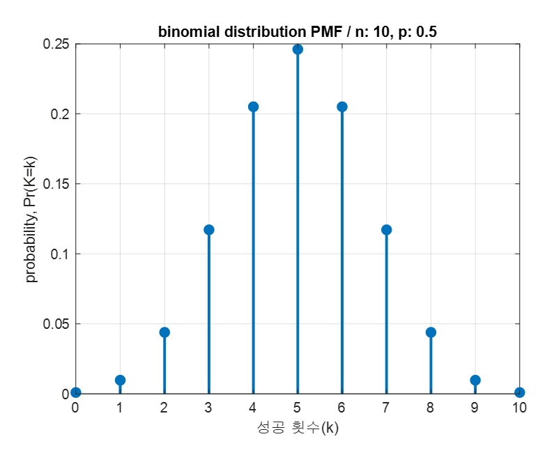
Figure 1. The binomial distribution showing the probability of various success counts with a total number of 10 trials and a success probability of 0.5.
Drawing a binomial distribution histogram through computer simulation (empirical probability)
One way to confirm the shape of the second binomial distribution is through computer simulation.
If you ask if you have to use a computer simulation… well, of course, you could conduct experiments directly, but it could take too much time. So let’s perform a simulation to confirm.
The method of performing the simulation is simple:
$\quad$ 1. Set the count of successes from 0 to 10 to 0.
$\quad$ 2. Toss the coin 10 times.
$\quad$ 3. Count how many times the coin landed heads (number of successes).
$\quad$ 4. Increase the success count of the corresponding success number. For example, if there were 3 successes, the count of 3 successes would increase by 1.
$\quad$ 5. Repeat steps 2 to 4 a large number of times (e.g., 100 times).
$\quad$ (Of course, the more repetitions, the closer the obtained values will be to the pre-determined probability distribution.)
The following video shows the simulation introduced in steps 1 to 5 performed directly and the count plotted in histogram form.
Figure 2. Shape of binomial distribution obtained through simulation
Characteristics of the Binomial Distribution
When dealing with the binomial distribution, important characteristics to know include the mean, variance, and under what conditions the binomial distribution resembles a normal distribution.
Mean and Variance of the Binomial Distribution
For a random variable K following a binomial distribution with total number of trials n and probability of success p,
the mean is
\[E(K) = np\]and the variance is
\[Var(K) = np(1-p)\]It is reasonable to think that if an event is conducted n times and the probability of success is p, then the number of successes should be around np. For example, it is reasonable to assume that if a coin is flipped 100 times, it will come up heads around 50 times.
A way to derive the mean is to use the linearity of expected value, which means that since the value of K obtained from each trial can be added together to obtain the total value of K,
\[K = K_1 + K_2 + \cdots + K_n\]it follows that
\[E[K] = E[K_1 + K_2 + \cdots + K_n] = E[K_1] + E[K_2] + \cdots + E[K_n]\]Since the expected value of K for each trial is p,
\[\therefore E[K] = \sum_{i=0}^n E[K_i] = \sum_{i=0}^n p = np\]The definition of variance is
\[Var(K) = \sum_i p_i(k_i-\mu)^2\]Like how the mean was derived above, if we think about each of the n trials, we can see that the possible outcomes k_i are either 1 or 0, with a probability of p for 1 and 1-p for 0.
Also, since the expected value when performed once is $\mu= p$, according to the definition of variance,
\[\Rightarrow (1-p)(0-p)^2+p(1-p)^2 = p^2(1-p) + p(1-p)^2\] \[= p^2-p^3 + p(1-2p+p^2) = p^2 -2p^2 + p\] \[= p(1-p)\]Therefore, since the variance of each trial is added up when the experiment is conducted independently n times,
\[\sigma_n^2 = \sum_{i=1}^n \sigma^2 = np(1-p)\]Normal Distribution Approximation of Binomial Distribution
If you play with the applet at the top of this posting, you can see that the shape of the binomial distribution sometimes looks similar to the bell-shaped normal distribution.
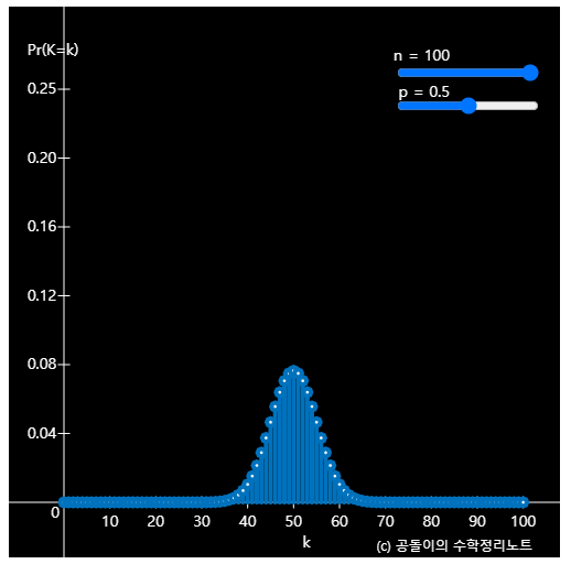
Figure 3. The shape of the binomial distribution is similar to that of the normal distribution.
However, in some cases, such as when n is too small or p is too small, it is difficult to say that the shape of the binomial distribution is similar to that of the normal distribution.
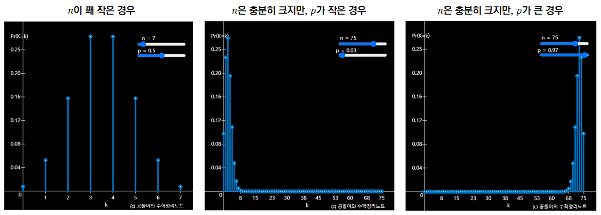
Figure 4. Three cases where it is difficult to say that the shape of the binomial distribution is similar to that of the normal distribution.
Looking at Figure 4, we can see that n should also be large and p should be around 0.5 to follow the shape of the normal distribution.
Mathematicians consider that the criteria for the binomial distribution to resemble the normal distribution are when $np$ and $\sqrt{np(1-p)}$ are both greater than 5, and then we can consider that the data follows the normal distribution with mean $np$ and variance $np(1-p)$.