Prerequisites

To understand the content of this post, it is recommended to have knowledge of the following:

• Elementary Square Matrices

Introduction to Triangular Matrices

To better understand the LU decomposition, it is helpful to briefly introduce the concept of triangular matrices.

In linear algebra, there is a type of matrix called a triangular matrix, which has a peculiar form. This matrix refers to a matrix whose upper or lower triangular elements, excluding the diagonal elements, are all 0 with respect to the main diagonal.

Therefore, a matrix with all upper triangular elements being 0 is called a lower triangular matrix, and a matrix with all lower triangular elements being 0 is called an upper triangular matrix.

• lower triangular matrix

\[L=\begin{bmatrix} l_{1,1} & & & & 0 \\ l_{2,1} & l_{2,2} & & & \\ l_{3,1} & l_{3,2} & \ddots & & \\ \vdots & \vdots & \ddots & \ddots & \\ l_{n,1} & l_{n,2} & \cdots & l_{n,n-1} & l_{n,n} \end{bmatrix}\]

• upper triangular matrix

\[U=\begin{bmatrix} u_{1,1} & u_{1,2} & u_{1,3} & \cdots & u_{1,n} \\ & u_{2,2} & u_{2,3} & \cdots & u_{2,n} \\ & & \ddots & \ddots & \vdots \\ & & & \ddots & u_{n-1,n} \\ 0 & & & & u_{n,n} \end{bmatrix}\]

Rethinking the solution to a system of equations

To represent the basic row operations used in the process of solving a system of equations with matrices, we considered Elementary Square Matrices.

To briefly recap, there are three types of elementary matrices:

1. Row multiplication
2. Row switching
3. Row addition

By using these elementary row operations, we can obtain solutions for each unknown variable. If we examine the system of equations from the bottom up, we can eliminate variables by reducing each equation to an expression containing only the last remaining unknown variable. For example, in the system of equations below,

\[\begin{cases}x+y+z = 6 \\ 2x+3y-z=5 \\ 2x+3y+3z=17\end{cases} % Equation (3)\]

we can perform the following operations:

\[r_2 \rightarrow r_2-2r_1 % Equation (4)\] \[r_3 \rightarrow r_3 - 2r_1 % Equation (5)\]

to obtain:

\[\begin{cases}x+y+z = 6 \\ 0x+y-3z=-7 \\ 0x+y+z=5\end{cases} % Equation (6)\]

Then, we can perform the following operation:

\[r_3 \rightarrow r_3- r_2 % Equation (7)\]

to obtain:

\[\begin{cases}x+y+z = 6 \\ 0x+y-3z=-7 \\ 0x+0y+4z=12\end{cases} % Equation (8)\]

Therefore, we can determine that $4z=12$ from the last equation, which means that $z=3$. We can then substitute $z=3$ into the second equation to obtain $y=2$, and substitute $y=2$ and $z=3$ into the first equation to obtain $x=1$.

The process of calculating from the last variable to the first variable is called back substitution.

Let’s represent back substitution with matrices.

What if we represent the process of finding the solution we calculated earlier using matrices?

In other words, we can express the equation in equation (3) as a matrix

\[\left[\begin{array}{ccc|c} 1 & 1 & 1 & 6 \\ 2 & 3 & -1 & 5 \\ 2 & 3 & 3 & 17\end{array}\right]% equation (9)\]

By performing elementary row operations such as those in equations (4), (5), and (7) on the matrix, we can obtain the matrix that represents the equation in equation (8):

\[\left[\begin{array}{ccc|c} 1 & 1 & 1 & 6 \\ 0 & 1 & -3 & -7 \\ 0 & 0 & 4 & 12\end{array}\right]\]

Let’s express the elementary row operations with elementary square matrices, which can be summarized as follows: Elementary Square Matrices.

\[\begin{bmatrix}1 & 0 & 0 \\ 0 & 1 & 0 \\ 0 & -1 & 1\end{bmatrix} \begin{bmatrix}1 & 0 & 0 \\ 0 & 1 & 0 \\ -2 & 0 & 1\end{bmatrix} \begin{bmatrix}1 & 0 & 0 \\ -2 & 1 & 0 \\ 0 & 0 & 1\end{bmatrix} \left[\begin{array}{ccc|c} 1 & 1 & 1 & 6 \\ 2 & 3 & -1 & 5 \\ 2 & 3 & 3 & 17\end{array}\right]= \left[\begin{array}{ccc|c} 1 & 1 & 1 & 6 \\ 0 & 1 & -3 & -7 \\ 0 & 0 & 4 & 12\end{array}\right]\]

If we consider the meaning of the elementary matrices that were applied to the left of the original $[A|b]$ matrix, they are the following elementary row operations:

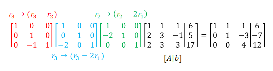
Figure 1. By performing elementary row operations, we can obtain the final result and perform back substitution.

Using the same method we used to find solutions for $x$, $y$, and $z$ above, we can find that $z=3$ by considering the result $4z=12$ from the right-hand side matrix. Similarly, we can find $y$ and $x$ in turn.

Now, let’s consider a slightly different approach using this idea. Instead of the augmented matrix $[A|b]$, we can use the same method by multiplying elementary matrices to the coefficient matrix $A$ without augmenting the right-hand side matrix. In this case, the resulting matrix will be in the form of an upper triangular matrix as introduced earlier.

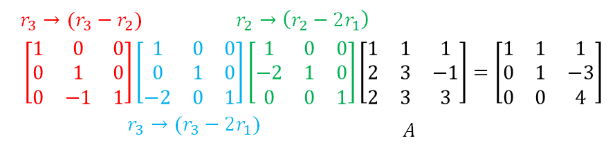
Figure 2. By performing elementary row operations, we can convert the coefficient matrix $A$ to upper triangular matrix form.

Multiplying the inverse matrix of a basic matrix: LU decomposition

As we learned in the time of Elementary Square Matrices, the inverse matrices of basic matrices have a very simple form. A brief review of them is as follows.

For example, the relationship between the row multiplication matrix and its inverse matrix is as follows:

\[E=\begin{bmatrix}1 & 0 & 0 \\ 0 & \color{red}{s} & 0 \\ 0 & 0 & 1\end{bmatrix} \rightarrow E^{-1}=\begin{bmatrix}1 & 0 & 0 \\ 0 & \color{red}{1/s} & 0 \\ 0 & 0 & 1\end{bmatrix}\]

Similarly, the relationship between the basic matrix that performs row addition and its inverse matrix is as follows:

\[E=\begin{bmatrix}1 & 0 & 0 \\ \color{red}{s} & 1 & 0 \\ 0 & 0 & 1\end{bmatrix}\rightarrow E^{-1}=\begin{bmatrix}1 & 0 & 0 \\ \color{red}{-s} & 1 & 0 \\ 0 & 0 & 1\end{bmatrix}\]

Also, the relationship between the basic matrix that performs the function of changing the order of rows and its inverse matrix is as follows:

\[P_{31}=\begin{bmatrix}0 & 0& \color{red}{1} \\ 0 & 1 & 0 \\ \color{blue}{1} & 0 & 0\end{bmatrix} \rightarrow P^{-1}_{31}=\begin{bmatrix}0 & 0& \color{red}{1} \\ 0 & 1 & 0 \\ \color{blue}{1} & 0 & 0\end{bmatrix}\]

Therefore, by multiplying the inverse matrices of the basic matrices that we had multiplied in front of the coefficient matrix A, as shown in Figure 2, in the order they were multiplied, we can rewrite the matrix A as shown below so that only A remains on the left side.

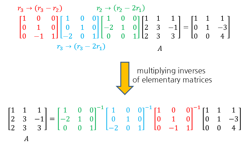
Figure 3. By multiplying the inverse matrices of basic matrices in order, we can leave only A on the left side.

Then, by directly calculating the inverse matrices of the basic matrices and combining them into one matrix through matrix multiplication, we can see that they can be combined into a lower triangular matrix, as shown in the following figure.

Therefore, we can divide the matrix A into the product of a lower triangular matrix and an upper triangular matrix.

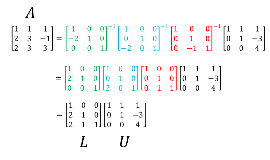
Figure 4. By calculating the inverse matrices of basic matrices and combining them, we can express matrix A as the product of a lower triangular matrix and an upper triangular matrix.

Using Substitution Matrices: PLU Decomposition

Some matrices may not be directly decomposed into LU form without row exchanges. The example of LU decomposition introduced earlier did not use row exchange operations. Let’s consider the LU decomposition, including row exchange operations.

For instance, consider the matrix $A$ below.

\[A = \begin{bmatrix}0& 0&3 \\ 1 & 1 & 1 \\ 2 & 3 & -1\end{bmatrix}\]

This kind of matrix cannot be transformed into an upper triangular matrix using only the basic matrices corresponding to row addition or row scaling in the basic form of a lower triangular matrix because the first row already has both elements 0.

Therefore, to use only the basic matrices corresponding to row addition and row scaling of a lower triangular matrix, we need to first change the rows of $A$.

In this example, let’s first exchange the first and third rows and then think about the LU decomposition. Therefore,

\[P_{13}=\begin{bmatrix}0 & 0 & 1 \\ 0 & 1 & 0 \\ 1 & 0 & 0\end{bmatrix}\]

If we multiply $P_{13}$ by $A$,

\[P_{13}A = \begin{bmatrix}2& 3&-1 \\ 1 & 1 & 1 \\ 0 & 0 & 3\end{bmatrix}\]

we get this matrix.

If we perform the operation $r_2\rightarrow r_2-(1/2)r_1$,

\[\Rightarrow \begin{bmatrix}1&0&0\\-1/2&1&0\\0&0&1\end{bmatrix}\begin{bmatrix}2& 3&-1 \\ 1 & 1 & 1 \\ 0 & 0 & 3\end{bmatrix}=\begin{bmatrix}2& 3&-1 \\ 0 & -1/2 & 3/2 \\ 0 & 0 & 3\end{bmatrix}\]

we see that it becomes an upper triangular matrix.

Therefore, we can consider the inverse of the elementary matrix of basic row operations and write it as follows:

\[P_{13}A = \begin{bmatrix}1&0&0\\-1/2&1&0\\0&0&1\end{bmatrix}^{-1}\begin{bmatrix}2& 3&-1 \\ 0 & -1/2 & 3/2 \\ 0 & 0 & 3\end{bmatrix}\] \[=\begin{bmatrix}1&0&0\\1/2&1&0\\0&0&1\end{bmatrix}\begin{bmatrix}2& 3&-1 \\ 0 & -1/2 & 3/2 \\ 0 & 0 & 3\end{bmatrix}= LU\]

That is, if we change the row order of the matrix $A$ to be decomposed in advance and perform the LU decomposition, we perform the PLU decomposition.

As mentioned earlier, the inverse matrix of the row exchange matrix is itself, so the original coefficient matrix $A$ can be decomposed as follows.

\[A=\begin{bmatrix}0& 0&3 \\ 1 & 1 & 1 \\ 2 & 3 & -1\end{bmatrix}\] \[=P_{13}LU = \begin{bmatrix}0 & 0 & 1 \\ 0 & 1 & 0 \\ 1 & 0 & 0\end{bmatrix}\begin{bmatrix}1&0&0\\1/2&1&0\\0&0&1\end{bmatrix}\begin{bmatrix}2& 3&-1 \\ 0 & -1/2 & 3/2 \\ 0 & 0 & 3\end{bmatrix}\]

Utilizing LU decomposition

Let’s think about the advantages of using LU decomposition.

Solving for Ax=b

Suppose A is a square matrix and can be factored as $A=LU$. Then, we can think of the following:

\[Ax=b\]

Since we can write $A=LU$,

\[\Rightarrow (LU)x=b\]

If we rearrange the parentheses as follows,

\[\Rightarrow L(Ux)=b\]

we can see that $Ux$ can also be thought of as a column vector. Therefore, if we substitute $Ux$ with a column vector named $c$,

\[\Rightarrow Lc=b\]

we get a problem in the form of the above.

However, if we carefully consider, $L$ is a lower triangular matrix and lower triangular matrices can easily obtain solutions using forward substitution.

Then, we can solve the problem of

\[Ux=c\]

to get the answer for $x$. In this case, using backward substitution makes it easy to obtain the solution.

For example, if we decompose the matrix A we saw above into LU, it would be as follows:

\[A=LU\] \[\Rightarrow\begin{bmatrix}1&1&1\\ 2& 3& -1\\ 2&3&3\end{bmatrix}= \begin{bmatrix}1 & 0 & 0 \\2& 1 & 0\\2 & 1 & 1\end{bmatrix} \begin{bmatrix}1 & 1 & 1 \\0& 1 & -3\\0 & 0 & 4\end{bmatrix}\]

Here, if $b$ in $Ax=b$ is given as $[6, 5, 17]^T$, then $LUx=b$ becomes

\[\begin{bmatrix}1 & 0 & 0 \\2& 1 & 0\\2 & 1 & 1\end{bmatrix} \begin{bmatrix}1 & 1 & 1 \\0& 1 & -3\\0 & 0 & 4\end{bmatrix} \begin{bmatrix}x\\y\\z\end{bmatrix}=\begin{bmatrix}6\\5\\17\end{bmatrix}\]

and if we convert the above equation into the form of $Lc=b$, we get

\[\begin{bmatrix}1 & 0 & 0 \\2& 1 & 0\\2 & 1 & 1\end{bmatrix} \begin{bmatrix}c_1\\c_2\\c_3\end{bmatrix}=\begin{bmatrix}6\\5\\17\end{bmatrix}\]

Then, we can easily find that $c_1=6$, $c_2=-7$, $c_3=12$, and considering that we need to solve the problem of $Ux=c$ additionally, we have

\[Ux=c\Rightarrow \begin{bmatrix}1 & 1 & 1 \\0& 1 & -3\\0 & 0 & 4\end{bmatrix}\begin{bmatrix}x\\y\\z\end{bmatrix} = \begin{bmatrix}6\\-7\\12\end{bmatrix}\]

Therefore, if we use back-substitution this time, we can know that $z=3$, $y=2$, and $x=1$.

Easy way to calculate determinant of a matrix

Similarly, if a matrix $A$ can be decomposed into LU, then we can think about the following:

\[A=LU\]

By the property of the determinant, we can obtain:

\[det(A)=det(L)det(U)\]

Since both $L$ and $U$ are triangular matrices, we can easily calculate the determinant of $A$ by taking the product of the diagonal elements.

In other words, if $L$ and $U$ are decomposed as in (1) and (2), then the determinant of $A$ can be calculated as follows:

\[det(A) = \prod_{i=1}^{n}l_{i,i}\prod_{j=1}^{n}u_{j,j}=\prod_{i=1}^{n}l_{i,i}u_{i,i}\]

This makes it easy to calculate the determinant of $A$.