Prerequisites
To understand surface integrals, it is recommended that you have knowledge of the following:
Formula for surface integrals
The formula for surface integrals can be written as follows:
\[\iint_S\vec{F}\cdot d\vec{S} = \iint_S\vec{F}\cdot\hat{n}dS\]Here, $\vec{F}$ is a vector field. Also, $\vec{S}$ is a surface vector, which can be expressed as $\hat{n}dS$ when broken down. In other words, its magnitude is the area of a small surface on the curved surface ($dS$), and its direction is the normal vector ($\hat{n}$) of the surface.
By examining the formula for surface integrals, we can also see that it is very similar to the formula for line integrals of vector fields.
For reference, the formula for line integrals of vector fields is as follows:
\[\int_C\vec{F}\cdot d\vec{r}\]The difference between line integrals of vector fields and surface integrals can be attributed to the difference in the range of the domain being integrated, whether it is a one-dimensional curve or a two-dimensional curved surface.
$dS$, the area of a small surface on the curved surface
In equation (1), the vector field $\vec{F}$ will be given in the problem, and the normal vector of a small surface on the curved surface $\hat{n}$ was covered in the previous article. Therefore, if we can learn more about the area $dS$ of a small surface on the curved surface, we will be able to calculate the surface integral.
In the article on normal vectors of surfaces, it was mentioned that there is a 3-dimensional output space corresponding to a 2-dimensional input space, and a 3-dimensional curved surface is determined by a mapping (i.e., function) called $r(t)$.
Furthermore, at any point on the surface, the rate of change with respect to a small change in the $u$ direction and a small change in the $v$ direction can be expressed as the following vectors, as shown in Figure 1:
\[\text{Rate of change of } r \text{ with respect to a small change in }u \Rightarrow \frac{\partial r}{\partial u} = r_u\]\(\text{Rate of change of } r \text{ with respect to a small change in }v \Rightarrow \frac{\partial r}{\partial v} = r_v\)
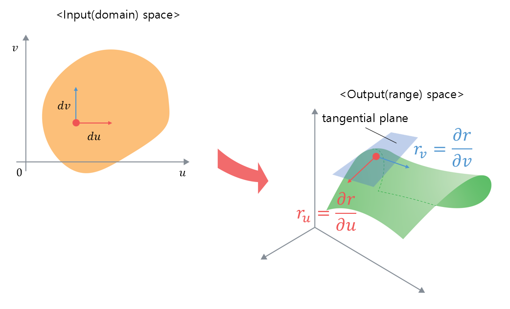
Figure 1. Rate of change in the output space with respect to small variations in the input space
Continuing the discussion in Figure 1, if we draw only the vectors shown in Figure 1 as in Figure 2 below:
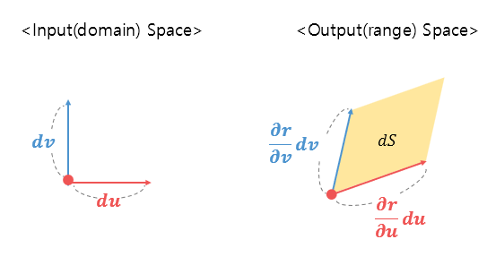
Figure 2. Rate of change in the output space with respect to small variations in the input space
If we look closely at the portion of the output space in Figure 2, we can see that the differential area $dS$ at the red point on the curved surface is marked.
The differential area $dS$ can be obtained by the changes in the $u$ direction and the $v$ direction of the $r$ vector. Since the two values, represented by partial derivatives, are both vectors, the size of the differential area $dS$ is
\[dS = \left|\left(\frac{\partial r}{\partial u}du\right)\times\left(\frac{\partial r}{\partial v}dv\right)\right|\]Here, since $du$ and $dv$ are scalar values, we can take the absolute value outside of the brackets:
\[=dudv\left|\frac{\partial r}{\partial u}\times\frac{\partial r}{\partial v}\right| = dudv|r_u \times r_v|\]If we expand the formula for surface integral,
In the previous session, we learned that the normal vector $\hat n$ of the differential surface can be expressed as follows:
\[\hat n = \frac{r_u \times r_v}{|r_u \times r_v|}\]Therefore, if we rewrite Equation (1), it will be as follows:
\[\iint_S\vec{F}\cdot\hat n dS = \iint_D\vec{F}\cdot \frac{r_u \times r_v}{|r_u \times r_v|}(dudv|r_u \times r_v|) = \iint_D\vec{F}\cdot(r_u \times r_v)dudv\]The reason why the subscript of the double integral sign has changed from $S$ to $D$ is that we integrate with respect to $u$ and $v$, and this is because the English expression for the domain is “Domain”.
That is, we transform the formula to be able to calculate it in the domain, which is equivalent to calculating it in the range.
Meaning of surface integral: 3D flux
The value of the surface integral represents the flow rate of the differential surface.
In the vector field’s flux (2D) article, we learned about the flow rate that can be obtained along a differential path. If we compare the flow rate along a differential path with the flow rate along a differential surface, it is shown in Figure 3 below.
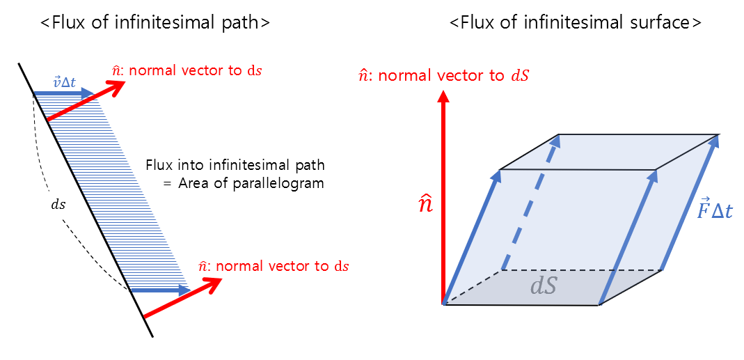
Figure 3. Comparison of flux along a small path and flux along a small surface
Let’s assume that a vector field $\vec{F}$ is given for the surface area $dS$ of a small surface.
Here, the assumption is that since the four sides of the small surface are very small in length, we assume that the vector field on the small surface is all the same.
Here, flux refers to the total amount of water that escapes in a unit time when the vector field represents the velocity of water.
If water escapes during time $\Delta t$, then the amount of water is equal to the volume of the parallelepiped shown on the right of Figure 3.
Since the velocity at which water escapes is $\vec{F}$, the length of the slope is $\vec{F}\Delta t$, and the height of the parallelepiped can be obtained by taking the dot product of $\vec{F}\Delta t$ with the normal vector $\hat n$.
Therefore, the total amount of water that escapes during time $\Delta t$ is
\[dS\times (\vec{F}\Delta t \cdot \hat n)\]and the amount of water that escapes per unit time is
\[dS\times (\vec{F}\cdot \hat n) = \vec{F}\cdot \hat n dS\]Integrating this over all surfaces by multiple integrals, we get
\[\iint_S\vec{F}\cdot \hat n dS\]which is equivalent to the surface integral in equation (1).
Therefore, we can say that the surface integral represents the total amount of flux that escapes along the surface $S$.