Prerequisites
To understand the Green’s theorem, it is recommended that you have knowledge of the following three concepts:
- Fundamental Theorem of Calculus
If a function $f$ is continuous on a closed interval $[a, b]$ and $F$ is an antiderivative of $f$, then the following holds:
\[\int_{a}^{b}f(t)dt = F(b) - F(a)\]Green’s Theorem
The Green’s theorem in the plane is as follows.
| THEOREM 1. Green’s Theorem |
|---|
| Let the vector field be given by $F(x,y) = P(x,y)\hat{i} + Q(x,y)\hat{j}$ and let the direction of the line integral be counterclockwise around the boundary of an area $A$. Then, |
As shown in the equation above, the left-hand side involves a double integral, while the right-hand side involves a line integral, and they are equal to each other.
In particular, one important aspect to note about Green’s theorem is that it is a theorem that applies to closed paths and their enclosed areas.
Proof of Green’s Theorem
In this post, we will prove Green’s theorem by first proving the line integral and then showing that its result is the same as that of the double integral.
Let us consider a closed path and its enclosed area as shown in the following figure.

Figure 1. Closed path $C$ and its enclosed area $A$ considered for the proof of Green's theorem.
Source: Mathematical Methods in the Physical Sciences, pp. 309, 3rd ed., Mary L. Boas
There are two ellipses in the figure, which represent the same closed curve with different parameterizations. From the left-hand side of Figure 1, $x$ varies from $a$ to $b$, and the lower and upper curves are denoted as $y_l$ and $y_u$, respectively.
On the right-hand side of Figure 1, $y$ varies from $c$ to $d$, and the left and right curves are denoted as $y_l$ and $y_r$, respectively.
We consider the following vector field:
\[\vec{F}(x,y)=P(x,y)\hat{i}+Q(x,y)\hat{j}\]We can now calculate the line integral as follows.
\[\oint_C\vec{F}(x,y)d\vec{r} = \oint_C\left(P(x,y)\hat{i}+Q(x,y)\hat{j}\right)(dx\hat{i}+dy\hat{j})\] \[=\oint_C P(x,y)dx + Q(x,y)dy\]Since the integration formula (5) is complicated to calculate at once, we will proceed with the calculation by adding the results for the $x$ and $y$ components separately when computing the integration of formula (5).
Integration with respect to $x$
Looking at the left ellipse of Figure 1, $x$ changes from $a$ to $b$ along the closed curve C, and the curve followed at that time can be thought of as divided into $y_l$ and $y_u$.
\[\oint_C P(x,y)dx\] \[=\int_{a}^{b}P(x,y_l)dx + \int_{b}^{a}P(x,y_u)dx\]Here, let’s reverse the order of $a$ and $b$ in the second integral formula of equation (7) and change the sign.
\[=\int_{a}^{b}P(x,y_l)dx - \int_{a}^{b}P(x,y_u)dx\] \[=\int_{a}^{b}P(x,y_l) - P(x,y_u)dx\]Using the fundamental theorem of calculus, we get the following.
\[=\int_{a}^{b}\int_{y_u}^{y_l}\frac{\partial P}{\partial y}dy\text{ }dx\]The reason why we used the fundamental theorem of calculus is that for any closed interval $[a,b]$ and continuous differentiable function $f$, we can think of it as
\[\int_{a}^{b}\frac{df}{dx}dx=f(b)-f(a)\]Formula (10) reverses the positions of $y_l$ and $y_u$ and adds a (-) sign.
The reason for reversing the positions of $y_l$ and $y_u$ is because the increasing direction of the $y$ axis goes from $y_l$ to $y_u$ as can be seen in Figure 1.
\[Formula (10) \Rightarrow -\int_{a}^{b}\int_{y_l}^{y_u}\frac{\partial P}{\partial y}dydx\] \[=-\iint_A\frac{\partial P}{\partial y}dxdy\](Even if the order of $dx$ and $dy$ is reversed during the double integration using Green’s theorem, it does not matter thanks to Fubini’s theorem.)
Integration with respect to $y$ component
Let’s now integrate with respect to the $y$ component.
Looking at the right ellipse in Figure 1, as we follow the closed curve C, $y$ changes from $c$ to $d$, and we can consider the curve followed at that time as divided into two parts, $x_l$ and $x_r$.
\[\oint_CQ(x,y)dy\] \[=\int_{d}^{c}Q(x_l, y)dy + \int_c^dQ(x_r,y)dy\]Similarly, let’s change the order of $c$ and $d$ and change the sign in the left integral of equation (15).
\[=-\int_{c}^{d}Q(x_l, y)dy + \int_c^dQ(x_r,y)dy\] \[=\int_c^d Q(x_r,y)-Q(x_l,y)dy\]Just like when integrating with respect to the $x$ component, we can use the fundamental theorem of calculus to obtain
\[=\int_c^d \int_{x_l} ^{x_r} \frac{\partial Q}{\partial x}dx dy\] \[=\iint_A\frac{\partial Q}{\partial x}dxdy\]Combining the results obtained for x and y components
If we consider the values of the line integrals with respect to the x and y components that we previously obtained, we can combine them to get the desired result according to Green’s theorem.
In other words,
\[Equation (5) = -\iint_A\frac{\partial P}{\partial y}dxdy + \iint_A\frac{\partial Q}{\partial x}dxdy\] \[= \iint_A\frac{\partial Q}{\partial x}-\frac{\partial P}{\partial y}dxdy\]This completes the proof of Green’s theorem.
Intuitive understanding of Green’s theorem through Curl
To understand the following content, it is recommended to know the following:
Let’s try to understand the intuitive meaning of Green’s theorem this time.
Suppose there is a region R with an area on a vector field as shown below.
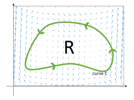
Figure 2: An arbitrary vector field $f$ and a closed curve C on the xy plane.
If we define the vector field $\vec{f}$ as
\[\vec{f}(x,y) = P(x,y)\hat{i}+Q(x,y)\hat{j}\]then, by Green’s theorem, the following equation holds:
\[\oint_C\vec{f}\cdot d\vec{r} = \iint_R\left(\frac{\partial P}{\partial y}-\frac{\partial Q}{\partial x}\right)dA\]The left-hand side of Equation (23) is the line integral of the vector field with respect to curve C.
The line integral value will be positive if the vector field flows along the curve in the counterclockwise direction and negative if the vector field flows mostly in the clockwise direction along the curve.
Now, let’s derive the right-hand side of Equation (23) from the left-hand side. Let’s split the region R in half as shown below.
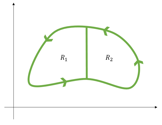
Figure 3: Let's divide region R in half. It doesn't matter whether we divide it vertically or horizontally.
Let’s call the closed curve of $R_1$ region $C_1$ and the closed curve of $R_2$ region $C_2$. Then the following holds:
\[\oint_{C_1}\vec{f}\cdot d\vec{r} + \oint_{C_2}\vec{f}\cdot d\vec{r} = \oint_{C}\vec{f}\cdot d\vec{r}\]Why is that? It’s because the line integrals calculated from $C_1$ and $C_2$ at the boundary between $R_1$ and $R_2$ cancel each other out. This is because line integrals fundamentally determine how much the vector field resembles the CCW direction.
Now, let’s divide $R$ into four equal parts as follows:
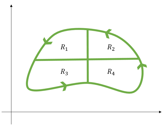
Figure 4. Dividing region R into four equal parts. It doesn't matter how you divide it, but for convenience, let's divide it as shown above.
Using the same logic as before, the following equation holds:
\[\oint_{C_1}\vec{f}\cdot d\vec{r} + \oint_{C_2}\vec{f}\cdot d\vec{r} + \oint_{C_3}\vec{f}\cdot d\vec{r} + \oint_{C_4}\vec{f}\cdot d\vec{r} = \oint_{C}\vec{f}\cdot d\vec{r}\]–
Then what happens when we divide region R into N equal parts? The following equation can be established:
\[\sum_{k=1}^{N}\oint_{C_k}\vec{f}\cdot d\vec{r} = \oint_{C}\vec{f}\cdot d\vec{r}\]Now, in order to consider equation (26), let’s briefly think about an arbitrary $k$th region when we divide region $R$ into N parts.

Figure 5. $N$th division of region $R$ into $N$ parts, considering $k$th region $R_k$.
As confirmed in the discussion about Curl, curl represents the rotational force experienced by a unit area. Therefore, when $N\rightarrow \infty$, the region $R_k$ can be considered as an infinitesimal area.
Then, what is the amount of rotation for the area $R_k$ with an area of $|R_k|$?
It is given by
\[\text{2d-curl}\left\{F(x_k,y_k)\right\}|R_k|\]In other words, this has the same meaning as
\[\oint_{C_k}\vec{f}\cdot d\vec{r}\]because the way we think about curl is to only consider the vectors that contribute to rotation in line integrals.
(If this is not immediately clear, I highly recommend reading the article on curl of a vector field.)
Therefore, equation (26) can be considered as follows:
\[\Rightarrow \oint_C\vec{f}\cdot d\vec{r}=\sum_{k=1}^{N}\oint_{C_k}\vec{f}\cdot d\vec{r}\approx \sum_{k=1}^{N}\text{2d-curl}\left\{F(x_k, y_k)\right\}|R_k|\]When $N$ is made infinitely large, $|R_k|\rightarrow dA$, and thus,
\[\oint_C\vec{f}\cdot d\vec{r} = \iint_R\text{2d-curl}\left\{\vec{f}\right\}dA = \iint_R\left(\frac{\partial P}{\partial y} - \frac{\partial Q}{\partial x}\right)dA\]is obtained.