Another perspective on differential equations

So far, we have explored various perspectives on interpreting differential equations.

In Modeling phenomena with differential equations, we defined differential equations as equations that involve derivative coefficients.

In Direction fields and Euler’s method, we geometrically interpreted differential equations using slopes mapped to coordinates $(x, y)$.

And in Euler’s number and homogeneous differential equations, we interpreted differential equations as systems with changing rates of continuous growth from a perspective of continuity.

These three interpretations have been very useful for interpreting differential equations numerically or analytically, and have served as important guideposts for understanding the characteristics of solutions to differential equations of not only first order, but also of higher degrees.

---

From now on, we will take another perspective on differential equations. Here, we will introduce the concepts of vectors and matrices used in linear algebra to functions.

From now on, we can treat functions as a type of vector, and the operations that correspond to matrices in linear algebra are extended as ‘linear operators’.

In addition, we will expand the concept of vector spaces, which are sets of vectors, to function spaces, which are sets of functions.

This logic has been precisely established as ‘functional analysis’, but in this post, we will briefly touch on the basic content.

Prerequisites

To understand this post, we recommend that you have a detailed understanding of the following topics. (In fact, you need to know all the basics of linear algebra to understand it well.)

• Basic operations of vectors (scalar multiplication, addition)
• Another perspective on matrix multiplication
• Meaning of row vectors and inner products of vectors
• Matrix and linear transformation
• Relationships among the four main subspace

functions as vectors

In a previous post on the basics of linear algebra, basic vector operations (scalar multiplication, addition), we thought of vectors from three perspectives.

They were defined as things like arrows, sequences of numbers, and elements of vector spaces.

Among them, the definition that a vector is an element of a vector space is the most mathematical definition, and I mentioned that this definition is important because it emphasizes that “things with these properties can all be treated as vectors and manipulated accordingly” in linear algebra.

In other words, if you discover a concept that has the properties of a vector, you can extend and apply the techniques and concepts that have been applied in linear algebra.

More specifically, to be a vector, a mathematical object (such as a vector, matrix, function, etc.) must be closed under the following two operations:

• Scalar multiplication of a vector
• Vector addition

Is it too simple?

Just like how by paying a membership fee for Netflix’s membership, you can enjoy all the videos provided by Netflix, if a mathematical object is found to satisfy only these two laws, it becomes a “vector” membership.

And accordingly, it can receive the concepts and techniques that have been hard-earned in linear algebra.

Figure 1. Benefits that can be enjoyed by subscribing to Netflix (Source: Netflix)

Although it is not a rigorous proof, just thinking briefly, a function qualifies as a vector.

Below is an expression of scalar multiplication and vector addition for functions.

\[(c\cdot f)(x) = c\cdot f(x) % 식 (1)\] \[(f+g)(x) = f(x)+g(x) % 식 (2)\]

In other words, if we multiply an arbitrary constant $c$ to a function $f(x)$, $cf(x)$ is still a function, and if we add two functions $f(x)$ and $g(x)$, $f(x)+g(x)$ is also a function.

Figure 2. The sum of two functions
Source: Function space, Wikipeda

Thus, just as vectors are defined as elements of vector spaces, functions can also be defined as vectors in a vector space, and the vector space that includes functions is called a “function space.”

---

We have discovered the concept of a function space by extending the concept of a vector.

The important point now is how to apply the concepts and techniques of linear algebra that apply to vectors to functions.

Once a concept has been extended, we must question everything we previously applied without any doubt.

This is because we can only think of the extended version of techniques after we have considered where the concept came from and what fundamental meaning it had.

Here, we will explore the “extended” versions of three linear algebra concepts in functional analysis.

Inner product of vectors → Inner product of functions

The first concept is the inner product operation.

In linear algebra, the inner product of two vectors is defined as follows.

For any $n$-dimensional real vectors $\vec{a}$ and $\vec{b}$ such as

\[\vec{a} = \begin{bmatrix}a_1\\ a_2 \\ \vdots \\ a_n\end{bmatrix} % Equation (3)\] \[\vec{b} = \begin{bmatrix}b_1\\ b_2 \\ \vdots \\ b_n\end{bmatrix} % Equation (4)\]

the dot product is defined as

\[\text{dot}(\vec{a}, \vec{b})=a_1b_1 + a_2b_2 +\cdots + a_nb_n % Equation (5)\]

If $\vec{a}$ and $\vec{b}$ were complex vectors, the inner product is defined as follows:

\[\text{dot}(\vec{a}, \vec{b})=a_1^*b_1 + a_2^*b_2 +\cdots + a_n^*b_n % Equation (6)\]

Here, $*$ denotes the complex conjugate operation.

The reason why complex vectors involve complex conjugate operation is to define the length of complex vectors through the inner product.

The magnitude of a real vector $\vec{a}$ (usually L2-norm) is defined as follows:

\[\text{norm}_2(\vec{a}) = \sqrt{a_1^2 + a_2^2 + \cdots + a_n^2} % Equation (7)\]

That is,

\[\text{norm}_2(\vec{a}) = \sqrt{\text{dot}(\vec{a}, \vec{a})}=\sqrt{a_1a_1+a_2a_2+\cdots+a_na_n} % Equation (8)\]

If we extend this concept to complex vectors, for a complex vector $\vec{a}$,

\[\text{norm}_2(\vec{a})=\sqrt{a_1^2+a_2^2 + \cdots a_n^2}=\sqrt{a_1^*a_1+a_2^*a_2+\cdots +a_n^*a_n}=\sqrt{\text{dot}(\vec{a},\vec{a})} % Equation (9)\]

must hold. Thus, the inner product operation of complex vectors should be defined as Equation (6).

Now let’s extend the method of Equation (6) to define the inner product of functions.

Since the functions used in dealing with differential equations may not be limited to the real function range and can have complex values, the definition of the inner product of complex vectors is extended as follows:

For any complex-valued functions $f$ and $g$ defined on the interval $(a, b)$ that have real input and complex output, the inner product $\langle f, g\rangle$ of two functions is defined as

\[\langle f, g\rangle \equiv \int_a^bf^*(x)g(x) dx % Equation (10)\]

Here, $f^*(x)$ denotes the complex conjugate of $f(x)$.

Matrix and Vector Multiplication → Relationship between Operator and Function

In the Matrix and Linear Transformation post, it was stated that a matrix is a type of function that operates on a vector.

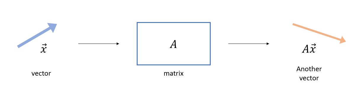
Figure 3. A matrix acts as a function that takes a vector as input and produces another vector as output.

If we think of general functions $f(x)$ and $g(x)$ as vectors, we can extend the concept of matrices in linear algebra to consider a function that takes another function as input and produces a different function as output.

We call such a concept an ‘operator’ that applies to functions. Like matrices in linear algebra, an operator takes a function as input and produces another function as output.

In particular, if an operator satisfies the following property, it is called a ‘linear operator.’ For any operator $L$,

\[L(\alpha f + \beta g) = \alpha Lf + \beta Lg % Equation (11)\]

where $\alpha$ and $\beta$ are arbitrary complex numbers and $f$ and $g$ are arbitrary complex functions.

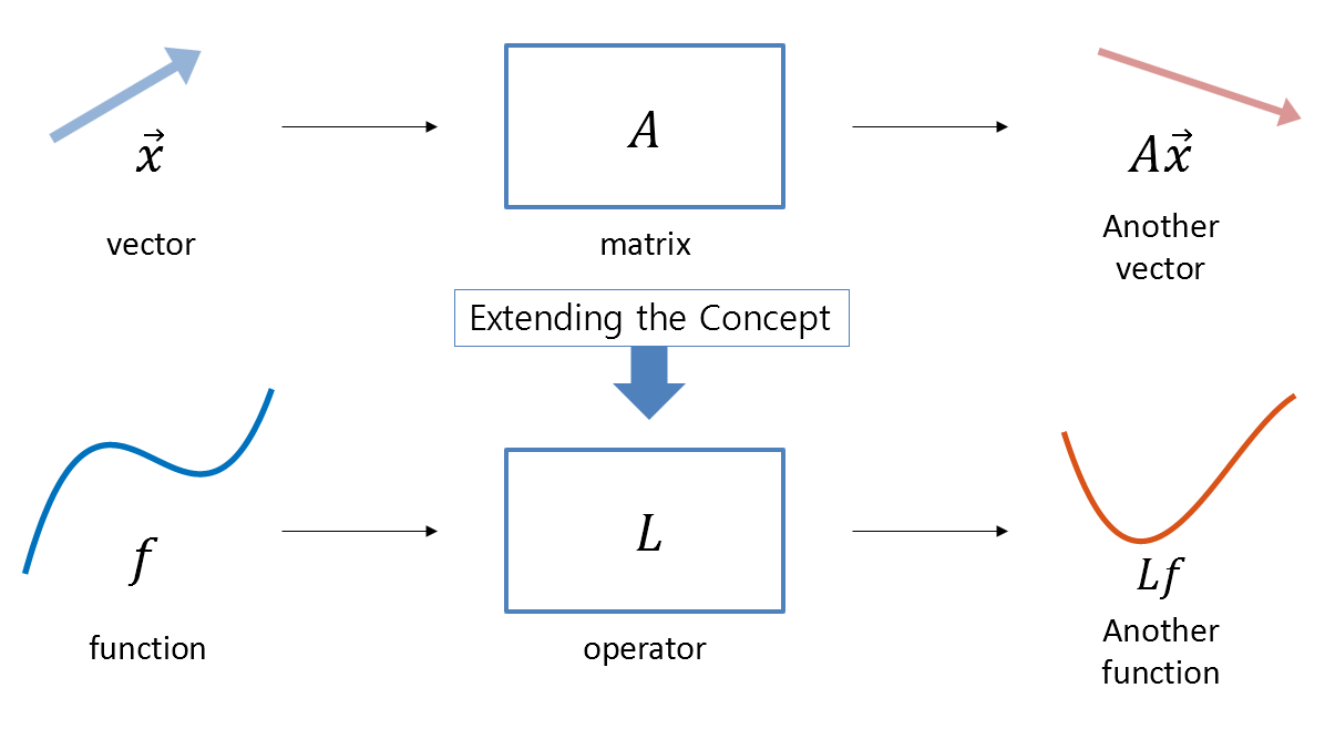
Figure 4. An operator is a function that takes a function as input and produces another function as output.

---

Continuing with abstract expressions for ‘operator’ can make it difficult to understand. Therefore, let’s consider some simple examples of operators below.

For an operator $L$ and function $\phi(x)$,

(1) Scalar multiplication operation

\[L\phi = \alpha \phi % Equation (12)\]

(2) Differential operator

The degree of differentiation can be any order.

\[L\phi = \frac{d^3}{dx^3}\phi \quad\text{ or }\quad L = \frac{d^3}{dx^3} % Equation (13)\]

Or multiple differentiation operations can be combined into one operator, and it is also possible to multiply another function and take a derivative.

For example, the following operator can be considered, and it is a linear operator.

\[L\phi = \phi^{(n)}(x)+a_1(x)\phi^{(n-1)}(x)+\cdots+a_{n-1}(x)\phi'(x)+a_n(x)\phi(x) % Equation (14)\]

That is, the operator is

\[L = \frac{d^n}{dx^n}+a_1(x)\frac{d^{n-1}}{dx^{n-1}}+\cdots+a_{n-1}\frac{d}{dx}+a_n(x) % Equation (15)\]

(3) Integral Operator

Not only can we take the integral of a function, but we can also multiply it by another function and integrate it. This is also a linear operator.

For any complex function $K(\cdot,\cdot)$,

\[L\phi = \int_{a}^{b}K(x, x')\phi(x')dx' % equation (16)\]

For example, convolution is also a type of integral operator.

\[L\phi = \int_{-\infty}^{\infty}g(x-x')\phi(x')dx' % equation (17)\]

Or Fourier transformation is also a type of integral operator.

\[L\phi = \int_{-\infty}^{\infty}e^{-2\pi i\xi x}\phi(\xi)d\xi % equation (18)\]

Transpose Operator → Adjoint Operator

Let’s think about the transpose operator this time.

The transpose operation for a vector is very simple. We just need to flip the rows and columns as follows:

\[\begin{bmatrix}1 & 2\end{bmatrix}^T = \begin{bmatrix}1\\2 \end{bmatrix} % equation (19)\]

So what was the role of the transpose operator in linear algebra?

The transpose operation changes a column vector to a row vector or a row vector to a column vector.

As we saw in the meaning of row vectors and inner products, a row vector is a functional that operates on a column vector.

By defining the transpose operation of a vector and considering the row vector as a function acting on a column vector, we can also compute the inner product of two vectors as follows:

For any vectors $\vec{a}$ and $\vec{b}$,

\[\vec{a}\cdot\vec{b} = \vec{a}^T\vec{b} % equation (20)\]

(Based on this background, mathematicians defined the operation between row vectors and column vectors as the dot product. This definition naturally extends to the definition of the product between matrices and vectors.)

In other words, by taking the transpose of $\vec{a}$, the original column vector becomes a row vector, and this allows the functionality of vectors to operate as operators.

The key point to be made here is that the transpose operation should be considered together with the dot product as an operation created to act on operators.

---

Now, let’s consider the dot product of two arbitrary vectors, where the second vector can be thought of as a vector transformed by a matrix $A$. In other words, for any two vectors $x$ and $y$, let’s consider the dot product

\[x\cdot Ay % Equation (21)\]

We will now consider the transpose operation of the matrix $A$ with this equation. According to Equation (20), we can express Equation (21) using the transpose operation as follows:

\[x^TAy % Equation (22)\]

If we rearrange the parentheses a bit, Equation (22) can also be expressed as:

\[(x^TA)y % Equation (23)\]

If we view this equation as the dot product of the vectors $x^TA$ and $y$, we can express Equation (23) using the transpose operation as follows:

\[(A^Tx)^Ty=(A^Tx)\cdot y % Equation (24)\]

Through what we have seen so far, let’s see how the transpose operation of vectors is extended to the function space¹.

The adjoint operation ($^\dagger$, read as dagger) with respect to the operator $L$ is a function that satisfies the following for two functions $\psi$ and $\phi$ and the operator $L$:

\[\langle \psi, L\phi \rangle = \langle L^\dagger \psi, \phi\rangle\]

Here, $\langle \psi, \phi \rangle$ is the inner product between $\psi$ and $\phi$.

---

Similar to explaining operators, let’s take a look at some examples rather than describing adjoints abstractly.

(1) Adjoint of Scalar Multiplication Operator

Consider the following operator for complex-valued functions $\phi$, $\psi$, $f$, $g$ defined on the interval $x\in [a, b]$ and any complex number $\alpha$.

\[L\phi = \alpha \phi\]

Then, $L^\dagger$ must satisfy the following.

\[\langle f, Lg\rangle = \langle L^\dagger f, g\rangle\] \[\langle f, Lg \rangle = \int_{a}^{b}f^*(x)Lg(x)dx=\int_{a}^{b}f^*(x)\alpha g(x)dx\] \[=\int_{a}^{b}(\alpha^*)^*f^*(x)g(x)dx=\langle a^*f, g\rangle\]

Thus, $L^{\dagger}$ is the operator defined as:

\[L^{\dagger}\psi = \alpha^*\psi\]

(where $^*$ denotes complex conjugate)

(2) Adjoint of Differential Operator

Consider the following operator for complex-valued functions $\phi$, $\psi$, $f$, $g$ defined on the interval $x\in [a, b]$.

\[L\phi = \frac{d}{dx}\phi\]

Then, $L^\dagger$ must satisfy the following.

\[\langle f, Lg\rangle = \langle L^\dagger f, g\rangle\] \[\langle f, Lg \rangle = \int_{a}^{b}f^*(x)Lg(x)dx=\int_{a}^{b}f^*(x) \frac{dg}{dx}dx\]

Using integration by parts, we can calculate as follows.

\[\Rightarrow f^*(x)g(x)\big |_{a}^{b}-\int_{a}^{b}\frac{df^*}{dx}g(x)dx\] \[= f^*(x)g(x)\big |_{a}^{b}+\int_{a}^{b}\left(-\frac{df^*}{dx}\right)g(x)dx\] \[=f^*(b)g(b)-f^*(a)g(a) + \left\langle -\frac{d}{dx}f, g\right\rangle\]

Thus, under the condition that $f^{\ast}(b)g(b) -f^{\ast}(a)g(a) = 0$, we can define the adjoint of the differential operator as:

\[L^{\dagger}\psi=-\frac{d}{dx}\psi\]

---

Also, let’s consider an operator that contains a second-order derivative as follows:

\[L\phi = p(x)\frac{d^2\phi}{dx^2}+q(x)\frac{d\phi}{dx}+r(x)\phi(x)\]

Then, $L^\dagger$ must satisfy the following.

\[\langle f, Lg\rangle = \langle L^\dagger f, g\rangle\]

From here on, for readability, let’s simplify the equation by omitting the symbol ‘$(x)$’ from the expressions.

\[\langle f,Lg \rangle = \int_{a}^{b}f^*\left\lbrace p\frac{d^2g}{dx^2}+q\frac{dg}{dx}+rg\right\rbrace\] \[=\int_{a}^{b}f^* p \frac{d^2g}{dx^2}dx + \int_{a}^{b}f^* q \frac{dg}{dx}dx+\int_{a}^{b}f^* r gdx\]

If we move the positions of $p(x)$, $q(x)$, and $r(x)$, we obtain:

\[\Rightarrow \int_{a}^{b}pf^* \frac{d^2g}{dx^2}dx + \int_{a}^{b}qf^* \frac{dg}{dx}dx+\int_{a}^{b}rf^* gdx\]

Among the three equations combined by addition in the above equation, if we calculate the first two equations separately, they are calculated as follows:

i)

\[\int_{a}^{b} p f^* \frac{d^2g}{dx^2}dx=(pf^*)\frac{dg}{dx}\Big |_{a}^{b}-\int_{a}^{b}\frac{d}{dx}\left(pf^*\right)\frac{dg}{dx}dx\] \[=(pf^*)\frac{dg}{dx}\Big|_{a}^{b}-\left\lbrace\frac{d}{dx}\left(pf^*\right)g\Big |_{a}^{b}-\int_{a}^{b}\frac{d^2}{dx^2}\left(pf^*\right)g dx\right \rbrace\] \[=(pf^*)\frac{dg}{dx}\Big|_{a}^{b}-\frac{d}{dx}(pf^*)g\Big|_{a}^{b}+\int_{a}^{b}\frac{d^2}{dx^2}(pf^*)g dx\]

ii)

\[\int_{a}^{b}qf^*\frac{dg}{dx}dx=(qf^*)g\Big|_{a}^{b}-\int_{a}^{b}\frac{d}{dx}(qf^*)gdx\]

Therefore, the original equation can be written as follows:

\[\Rightarrow \left(pf^*\frac{dg}{dx}-\frac{d}{dx}(pf^*)g+(qf^*)g\right)\Big|_{a}^{b}+\int_{a}^{b}\frac{d^2}{dx^2}(pf^*)g-\frac{d}{dx}(qf^*)g+rf^*g dx\]

Here, if we denote the left-hand side of the equation as $J(f, g)$, then we have:

\[\Rightarrow J(f, g)+\left\langle \left(\frac{d^2}{dx^2}p^*(x)-\frac{d}{dx}q^*(x)+r^*(x)\right)f, g\right\rangle\]

Therefore, under the condition that $J(f,g)=0$, we can find the following $L^{\dagger}$:

\[L^{\dagger}\psi=\frac{d^2}{dx^2}\Big(p^*(x)\psi(x)\Big)-\frac{d}{dx}\Big(q^*(x)\psi(x)\Big)+r^*(x)\psi(x)\]

$Ax=b$ in the world of functions

In this post, we have examined the characteristics of functions as vectors and the operations that can be applied to them by realizing that functions can be viewed as a kind of vector.

Just as linear algebra studies the process of finding a solution $x$ for $Ax=b$ with matrix $A$ and vectors $x$ and $b$, we can consider understanding the process of finding a solution $u$ for $Lu=f$ with operator $L$ and functions $u$ and $f$ as the ultimate goal of treating functions as vectors.

So, under what conditions did a solution for $Ax=b$ exist in linear algebra?

Existence of solution of $Ax =b$

As we saw in another perspective on matrix multiplication, a solution existed when $b$ was in the column space of $A$.

This can be explained from another perspective using the relationship between the major subspace (row space, column space, null space, left null space) to consider the conditions for the existence of a solution.

Let us consider some vector $y$ that satisfies the following condition.

\[A^Ty=0\]

Then, let us take the dot product of $x$ and $y$ for the original equation $Ax=b$.

\[Ax\cdot y = (Ax)^Ty = x^TA^Ty\]

We can think of the expression differently by rearranging the parentheses as follows:

\[\Rightarrow x^T(A^Ty)\]

Since we have the relationship $A^Ty=0$, we have

\[x^T(0) = 0\]

However, by the relationship $Ax=b$, we also have $(Ax)^Ty=b^Ty$, and since we have confirmed that $(Ax)^Ty=0$, we have $b^Ty=b\cdot y = 0$. Therefore, we can see that $\vec{b}$ and $\vec{y}$ are orthogonal vectors.

However, if we think a little bit, we can see that $y$ is a vector in the left null space, according to the definition of the left null space.

And as we learned in the relationship between the four main subspaces, the column space is always orthogonal to the left null space.

Therefore, if the $b$ vector is orthogonal to $y$, then the $b$ vector is in the vector space orthogonal to the left null space and we can know that $b$ is a vector in the column space.

Thus, the condition for the existence of a solution to $Ax=b$ is that for $y$ satisfying $A^Ty=0$, $b^Ty=0$.

Solvability of $Lu = f$

We have looked at the adjoint $L^\dagger$ of the operator $L$ in the function space.

If we apply the discussion above in linear algebra directly to the function space, the condition for $Lu=f$ to have a solution is as follows.

Let’s take the inner product of $v$ with $Lu=f$, where $v$ is a function satisfying $L^\dagger v=0$.

Then,

\[\langle v, Lu\rangle = \langle v, f\rangle\]

By the definition of the adjoint, the above equation can be written as follows.

\[\langle L^\dagger v, u\rangle = \langle v, f\rangle\]

Since $L^\dagger v=0$, the left-hand side of the above equation becomes 0. Therefore,

\[\langle v, f \rangle = 0\]

This means that, similar to the condition for the existence of a solution to $Ax=b$ in linear algebra above, the condition for $Lu=f$ to have a solution in the function space is that the function $f(x)$ is orthogonal to the null space of the adjoint operator.

This theory is also called one of the Fredholm theorems, the Fredholm alternative.

References

• function space, Wikipedia (https://en.wikipedia.org/wiki/Function_space)
• Applied Mathematical Methods in Theoretical Physics, 2nd ed., Wiley-VCH, Michio Masujima
• Advanced Differential Equations: Asymptotics & Perturbations, Arxiv, 2020, J Nathan Kutz