Prerequisites

To understand this post, you need to have prior knowledge of the following:

• Convolution of Discrete Time Signals
  • Convolution operation
  • Concept of impulse response
• FIR filter
• Basic knowledge of matrix operations (matrix multiplication, inverse matrix, etc.)

Impulse response and convolution of signals

Understanding impulse response is essential to comprehend this post.

If necessary, briefly understand the impulse response before continuing to read this post.

If you believe you have sufficient understanding of the impulse response, you can skip this part.

Let’s consider an arbitrary discrete signal $x[n]$ in the following form.

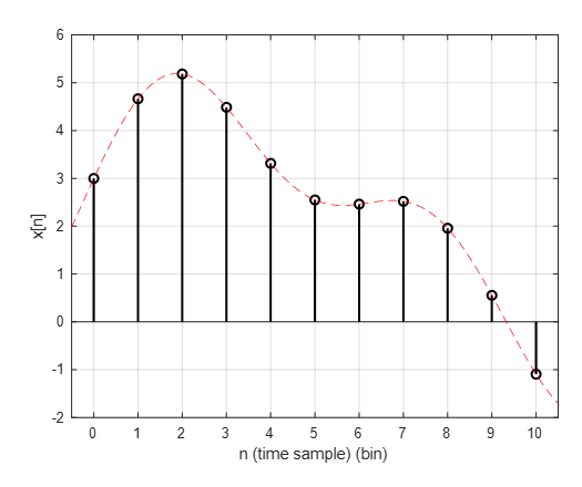
Figure 2. Arbitrary discrete signal $x[n]$

Note that the red dashed line can be thought of as the original function before time sampling.

The discrete signal $x[n]$ can also be seen as a list of $x[n]$ values for all integers $n$. However, since these values must appear in chronological order, they can also be seen as a linear combination of impulses, each having a function value of $x[n]$ as shown in the following figure.

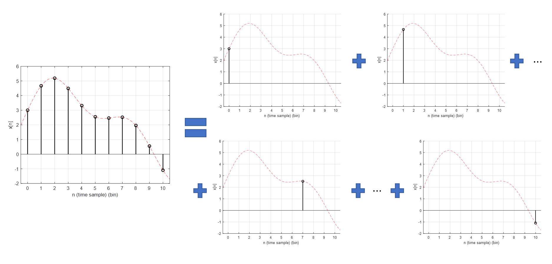
Figure 3. Arbitrary discrete signal $x[n]$

The equation for Figure 3 can be expressed as follows.

\[x[n] = \cdots + x[-2]\delta[n+2]+ x[-1]\delta[n+1] + x[0]\delta[n+0] + x[1]\delta[n-1] + + x[2]\delta[n-2]+\cdots\] \[=\sum_{k=-\infty}^\infty x[k]\delta[n-k]\]

Here, $\delta[n]$ is a function defined as follows:

\[\delta[n] = \begin{cases} 1 && \text{ if}\quad n = 0 \\ 0 && \text{otherwise } \end{cases}\]

Let’s consider a linear system. Let the input to this system be $x[n]$ and the output be $y[n]$. If we think of the linear system that connects the output and input as a linear operator $O_n(\cdot)$, then we can think of the input-output relationship as follows. (Here, the subscript $n$ of $O_n$ means that this operator is an operator for $n$.)

\[y[n] = O_n(x[n])\]

If we substitute Equation (1) into Equation (4), we get:

\[\Rightarrow O_n\left(\sum_{k=-\infty}^\infty x[k]\delta[n-k]\right)\]

Here, $O_n(\cdot)$ is a linear operator for $n$, so we can treat $x[k]$ as a constant. Therefore,

\[\Rightarrow \sum_{k=-\infty}^{\infty}x[k]O_n\left(\delta[n-k]\right)\]

Let’s define $O_n(\delta[n])$ as $h[n]$.

$h[n]$ is called the impulse response.

Then,

\[\Rightarrow \sum_{k=-\infty}^{\infty}x[k]h[n-k]\]

Suppose the length of the impulse response $h[n]$ is finite, as follows:

\[h[n] = \begin{cases} h[n] && \text{ if } -M\leq n \leq M \\ 0 && \text{otherwise}\end{cases}\]

Then, we can express $y[n]$ of Equation (7) as follows:

\[y[n] = \sum_{k=-M}^{M}x[k]h[n-k]\]

A system whose impulse response has a finite length like this is called a Finite Impulse Response (FIR) system.

Smoothing of signals using polynomial regression models

There are various methods for smoothing signals.

One representative smoothing method is the moving average, which calculates the average of a portion of the entire data sequentially through windowing rather than the mean of the entire data when time series data is arranged, and represents the mean value as the representative value of the window. This method is called smoothing the data.

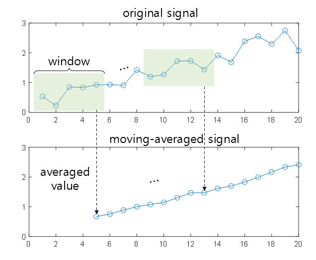
Figure 2. Operation principle of moving average

Taking a moving average can also be thought of as convolving the signal with the impulse response shown below. For example, for an M-order moving average, the impulse response is as follows.

\[h[n] = \begin{cases}1/M && \text{ for } n = 0, 1, \cdots, M-1 \\0 && \text{otherwise} \end{cases}\]

One disadvantage of the moving average is that it uses the mean value, which is known to be highly sensitive to outliers. Therefore, in some applications, the median value is used instead of the mean value.

Although the moving average has the advantage of being easy to implement, it has limitations that are vulnerable to instantaneous peaks.

One way to complement this is to construct a polynomial regression model for a short signal interval within the window applied to the time series and use it to smooth the signal.

Figure 3. Smoothing process of the signal using a polynomial regression model
Image source: Wikipedia Savitzky Golay filter

The figure above shows the process of smoothing the signal by constructing a polynomial regression model within a short window interval.

Even if using a polynomial regression model to smooth the signal is meaningful, the process of calculating the regression equation for each interval can be very time-consuming and inefficient.

The Savitzky-Golay filter (S-G filter) suggests that it is possible to mathematically replace smoothing using a polynomial regression model precisely without calculating the regression model at each time step within the window by preparing a specific impulse response for smoothing with the regression model.

In other words, by using a properly calculated impulse response, it is possible to design a filter that can achieve the same effect as calculating a regression model for every window at each time step, and this is what the S-G filter is suggesting.

Derivation

Assuming all signals to be discussed from now on are digital signals, let us denote the time sample as $n$ going forward.

What we want to do is to replace the signal $x[n]$ within the range of $-M\leq n \leq M$ with an appropriate $N$th order regression model $p(n)=\sum_{k=0}^{N}a_kn^k$.

In other words, the signal $p(n)$ obtained by smoothing using the regression model is as follows:

\[p(n) = a_0 + a_1 n+ a_2 n^2 + \cdots a_Nn^N\]

To be more specific, we acquire $2M+1$ signals with a length of $2M+1$ by obtaining $-M$ signals to the left and $+M$ signals to the right of the time sample 0, and replace them with an $N$th order regression model.

The reason we analyze the signal centered on the value of time sample 0 is that we ultimately want the impulse response needed when using the regression model for smoothing. By convolving the original signal with the impulse response, smoothing can ultimately be performed.

Now, the most appropriate regression model $p(n)$ that models this signal with a length of $2M+1$ will be composed of coefficients $a_k\text{ where }k =0 ,1 ,\cdots, N$ that minimize the error with the original signal as follows.

\[\epsilon_N = \sum_{n=-M}^{M}\left(p(n)-x[n]\right)^2\] \[=\sum_{n=-M}^{M}\left(\sum_{k=0}^Na_kn^k - x[n]\right)^2\]

By partial differentiation, we can find the coefficients $a_i\text{ for }i=0,1,\cdots,N$ that minimize the error.

\[\frac{\partial\epsilon_N}{\partial a_i}=\sum_{n=-M}^{M}2\left(\sum_{k=0}^{N}a_kn^k-x[n]\right)n^i = 0\notag\] \[\text{ for }i=0,1,\cdots,N\]

By simplifying the above equation, we get

\[\sum_{n=-M}^{M}n^i\sum_{k=0}^{N}a_kn^k-\sum_{n=-M}^{M}n^ix[n] = 0\] \[\Rightarrow \sum_{n=-M}^{N}\sum_{k=0}^{N}n^{i+k}a_k=\sum_{n=-M}^{M}n^ix[n]\]

Now, let’s define the following matrix $A$ to represent equation (15) using matrices.

$(2M+1)\times(N+1)$의 dimension을 갖는 어떤 행렬 $A$를 다음과 같이 정의하도록 하자.

\[A = \lbrace a_{n, i} \rbrace = \lbrace n^i \rbrace\notag\] \[\text{where }-M\leq n \leq M \text{ and } i=0,1,\cdots,N\]

Here, the notation $\lbrace a_{n,i}\rbrace$ indicates that the element in the $i$th column of the $n$th row is defined as $n^i$.

For reference, if we write the elements of $A$ individually, the matrix looks like the following ¹.

\[A = \begin{bmatrix} (-M)^0 && (-M)^1 && \cdots && (-M)^N \\\\ (-M+1)^0 && (-M+1)^1 && \cdots && (-M+1)^N \\\\ \vdots && \vdots && \vdots && \vdots \\\\ 0^0 && 0^1 && \cdots && 0^N \\\\ 1^0 && 1^1 && \cdots && 1^N \\\\ \vdots && \vdots && \ddots && \vdots \\\\ M^0 && M^1 && \cdots && M^N \end{bmatrix}\]

Also, in order to express Equation (15) using matrices, we need to introduce a few additional vectors, which are:

\[\vec a = [a_0, a_1, a_N]^T\] \[\vec x = [x[-M], \cdots, x[-1], x[0], x[1], \cdots, x[M]]^T\]

Using $A$, $\vec{a}$, and $\vec{x}$, we can express Equation (x) as follows:

\[Equation(15)\Rightarrow A^TA\vec{a} = A^T \vec{x}\]

To better understand this process, if we calculate $A^TA$, the $i$th row of $A^T$ and the $k$th column of $A$ are:

\[A^T_{(i,:)}=[(-M)^i, (-M+1)^i, \cdots, M^i]\] \[A_{(:, k)} = [(-M)^k, (-M+1)^k, \cdots, M^k]^T\]

Therefore, the $(i,k)$th element of $A^TA$ is:

\[A^TA = \lbrace a_{i,k}\rbrace = \left\lbrace \sum_{n=-M}^{M}(n)^{i+k}\right\rbrace\]

Moreover, we can compute $A^T\vec{x}$ as follows.

\[A^T\vec{x}=\begin{bmatrix} (-M)^0 && (-M+1)^0 && \cdots && 0^0 && 1^0 && \cdots && M^0 \\\\ (-M)^1 && (-M+1)^1 && \cdots && 0^1 && 1^1 && \cdots && M^1 \\\\ \vdots && \vdots && \vdots && \vdots && \vdots && \vdots && \vdots \\\\ (-M)^N && (-M+1)^N && \cdots && 0^N && 1^N && \cdots && M^N \end{bmatrix} \begin{bmatrix}x[-M]\\ \vdots \\ x[-1] \\ x[0] \\ x[1] \\ \vdots \\ x[M]\end{bmatrix}\] \[=\begin{bmatrix}\sum_{n=-M}^{M}n^0x[n] \\\\\sum_{n=-M}^{M}n^1x[n] \\\\ \vdots \\\\\sum_{n=-M}^{M}n^Nx[n]\end{bmatrix}\] \[=\sum_{n=-M}^{M}\begin{bmatrix}n^0 \\n^1 \\ \vdots \\ n^N \end{bmatrix}x[n]\]

Then, we can calculate the coefficient vector $\vec{a}$ through Equation (20) ².

\[\vec{a} = (A^TA)^{-1}A^Tx\]

Thus, we can summarize the result as follows.

\[(A^TA)^{-1}A^Tx = Hx\]

Therefore, we can calculate the first coefficient $a_0$ as follows.

\[a_0 = H_{(1,:)}\cdot \vec{x}=\sum_{m=-M}^{M}h_{1, m}x[m]\]

Here, $H_{(1,:)}$ represents the first row of $H$.

Now, if we think about Equation (29) again, we can see that it is equal to the output $y[n]$ at $n=0$ for a finite length signal $x[n] \text{ for } -M\leq n \leq M$.

In other words,

\[Equation (29)\Rightarrow y_0 = a_0 = \sum_{m=-M}^{M}h[0-m]x[m]\]

Comparing Equation (30) and Equation (9), which describes the input and output of a system with a finite impulse response, we can see that the first row of $H$ we obtained is the impulse response of the Savitzky-Golay filter.

MATLAB Code

clear; close all; clc;

M = 10; % The length of the filter is 2M+1 = 21
N = 9; % The degree of the polynomial is 9

% Test signal
load mtlb
t = (0:length(mtlb)-1)/Fs;

%% Obtaining coefficients with MATLAB
b = sgolay(N, 2*M+1);

sgolay_filter = b((size(b,1)+1)/2,:);

smtlb = conv(mtlb, sgolay_filter,'same');

%% Directly performing convolution with MATLAB
smtlb_MATLAB = sgolayfilt(mtlb, N, 2*M+1);

%% Computing S-G filter coefficients directly
A = zeros(2*M+1, N+1);

n_range = -M:M; % n in the original paper
i_range = 0:N; % i in the original paper
for i = 1:size(A,1)
    for j = 1:size(A,2)
        A(i,j)= n_range(i)^i_range(j);
    end
end

% matrix H = (A^TA)^{-1}*A^T

H = (A'*A)\A';

sgolay_filter_calculated = H(1,:); % The first row of H is the impulse response of the S-G filter.

my_smtlb_calculated = conv(mtlb, sgolay_filter_calculated,'same');

figure;
h1 = plot(t, mtlb);
axis([0.2 0.22 -3 2])
hold on;
% plot(t, smtlb);
h2 = plot(t, my_smtlb_calculated,'r', 'linewidth',2);
% plot(t, smtlb_MATLAB);
legend([h1, h2], 'Original signal','S-G filter applied')

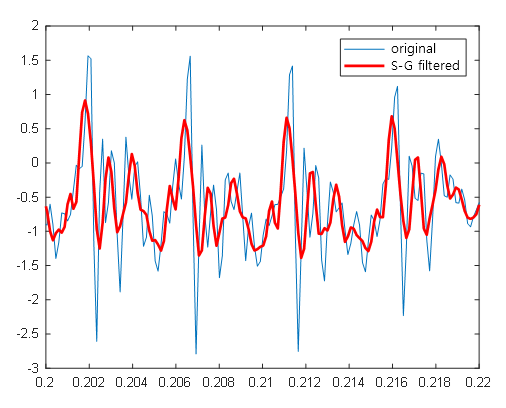
Figure 4. Result of running the above MATLAB code

Comparison with Moving Average

S-G filter is known to preserve the overall trend of the waveform better than the moving average filter. The example below shows the difference between the smoothing results of the moving average filter and the S-G filter.

In the figure below, if there were no noise in the black signal, it would have been a box-shaped function. However, the S-G filter produces a result that is closer to a box-shaped function after smoothing.

Figure 5. Comparison of smoothing results between Moving Average and S-G filter
Figure source: On Employing a Savitzky-Golay Filtering Stage to Improve Performance of Spectrum Sensing in CR Applications Concerning VDSA Approach

References

• What is a Savitzky-Golay Filter, IEEE, 2011, Ronald W. Schafer