This post is written based on the content provided by ZyBooks in University of California Davis ENG 006: Engineering Problem Solving.

Prerequisites

To better understand the content of this post, it is recommended to be familiar with the following topics.

• Elementary Square Matrices
• LU Decomposition

Introduction

Through the previous posts on Elementary Square Matrices and LU Decomposition, we confirmed that we can solve a system of linear equations using matrix form. In this case, the basic matrices (usually denoted as $E$) corresponding to elementary row operations played a crucial role.

That is, our goal is to change $Ax=b$ to $Ux=c$ by performing basic row operations.

Here, $U$ is an upper triangular matrix.

If we can transform $Ax=b$ to the form of $Ux=c$, we can study how to easily solve unknown variables $x_1, x_2,$ and $x_3$ using back-substitution.

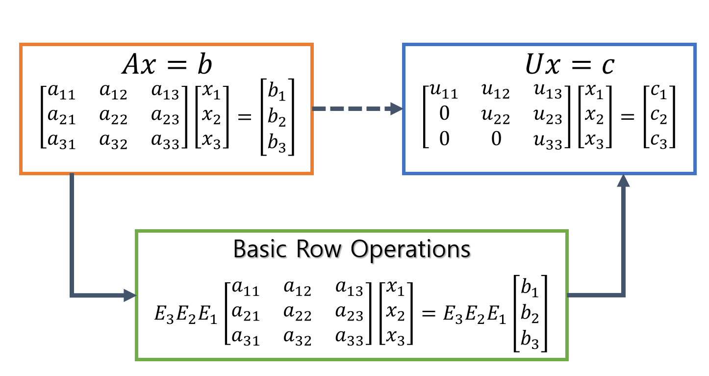
Figure 1. The process of obtaining an upper triangular matrix through basic row operations.

In LU Decomposition, when applying the above method, the matrix $A$ was a square matrix of size $n \times n$.

However, it is not necessary for matrix $A$ to be a square matrix of size $n \times n$ in order to perform row operations like the above.

In other words, there may be cases where the number of equations is less than the number of variables, or where the number of equations is greater than the number of variables. Can we still obtain something similar to an upper triangular matrix in these cases?

Also, if we eliminate all the numbers above the diagonal elements rather than obtaining an upper triangular matrix, what will happen?

LU Decomposition and REF, RREF

※ REF stands for Row-Echelon Form and RREF stands for Reduced Row-Echelon Form.

For a rectangular matrix, we can obtain a row-echelon matrix by performing row operations, just like performing LU decomposition to obtain an upper triangular matrix.

Roughly speaking, we can say that the row-echelon matrix has the following form:

Figure 2. The expected result obtained by performing row operations on a rectangular matrix

We call a matrix like the one in Figure 2 a row-echelon matrix or the row-echelon form of a given matrix. In Korean, it is called a “ladder matrix,” but I will refer to it as a row-echelon matrix since the term in Korean is somewhat misleading. In Figure 2, the triangles (▲) and hyphens (-) both represent non-zero elements. Moreover, we call the triangle (▲), which is the leading coefficient of a non-zero row, a pivot, and we call the column that contains the pivot a pivot column.

Now that we have grasped the terminology, let’s summarize the properties of a row-echelon matrix:

• All non-zero rows are above any rows of all zeros (i.e., all zero rows are at the bottom of the matrix).
• The leading coefficient of a non-zero row is always to the right of the leading coefficient of the row above it.
• All entries in a pivot column below the pivot are zero.

Although it may be confusing to read, the above means that a row-echelon matrix has a staircase-like shape as shown below.

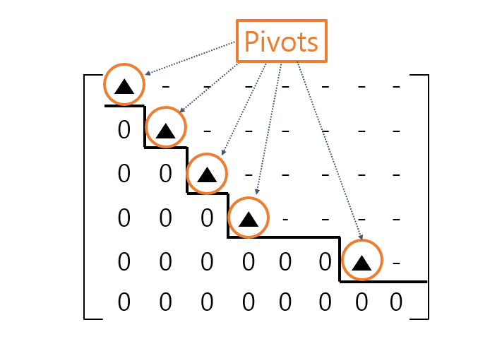
Figure 3. A row-echelon matrix has a staircase-like shape, and the part where the foot touches and goes up to each step is called a pivot.

In other words, a row-echelon matrix is a matrix obtained by performing row operations on a rectangular matrix $A$ and has a form and function similar to that of an upper triangular matrix. It must satisfy the three properties mentioned above. Therefore, we can obtain it by continuously performing row exchanges to make it have the desired form while performing row operations.

And if you scale the pivots to 1 and make all the numbers above the pivots 0, the row-echelon form in the form of Figure 3 can also be transformed as follows.

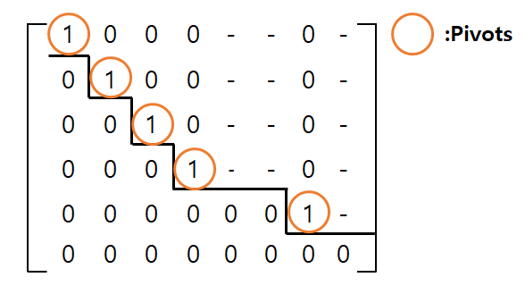
Figure 4. If you scale all the pivots to 1 and make all the numbers above the pivots 0 in the row-echelon form, it becomes the reduced-row echelon form.

Examples of REF & RREF: Distinguish them visually

The concept of row-echelon matrix can be confusing when you first encounter it. This is because the characteristics of a row-echelon matrix written in words may not be easy to understand. So let’s check if a matrix is a row-echelon matrix with some examples.

REF means Row-Echelon Form and RREF means Reduced Row-Echelon Form.

The following matrix can be considered as a REF.

Here, ‘-‘ denotes a non-zero number.

The following matrix can also be considered as a REF. It is not a requirement that the first term of the first row must be a non-zero term.

However, the following matrix is not a REF because it violates the rule that a row consisting only of 0’s should be located at the bottom.

Also, a matrix in the following form is not a REF. This is because it violates the second of the three characteristics, namely, the non-zero leading coefficient of the second row is to the left of the non-zero leading coefficient of the first row.

Furthermore, the following matrix is not in REF. This is because all terms below the pivot of 4 in the second column are not represented as 0.

The following matrix can be considered as RREF.

However, the following matrix is not RREF. According to the definition of pivot, the 4 in the second row and second column is a pivot of the row, but if it is RREF, all pivots should be 1.

If you multiply all terms of the second row by 1/4, it becomes RREF.

Finding REF & RREF by Hand

Finding REF and RREF by Hand

Let’s perform elementary row operations on the matrix $A$ below to obtain a row-echelon matrix.

Perform the following row operations:

Then, we can obtain the following matrix:

Up to this point, this is the row-echelon form of the matrix $A$.

Let’s multiply the second row by 1/4 and the third row by 1/2.

That is,

After these operations, the matrix is modified as follows.

Here are two row operations to make all values above the pivot zero, as well as below it.

As a result, we obtain the following matrix:

This is the reduced-row echelon form of matrix A.

Finding REF and RREF in MATLAB

Through MATLAB or other computational tools for linear algebra, we can calculate the Row Echelon Form (REF) or Reduced Row Echelon Form (RREF) of a given matrix.

However, the REF is not uniquely determined. For example, when calculating the REF of a matrix, we can still regard it as an REF even if we do not reduce the pivot value.

For example, for the matrix $A$ below,

One of the REFs can be the following:

However, we can still recognize it as an REF even if we multiply 1/2 to the second row.

Therefore, although REF is not uniquely determined, in MATLAB, we can obtain a similar result to REF using the lu function used in LU decomposition.

If we enter the command as follows in MATLAB,

A = [1, 1, 2, 3, 4; 2, 6, 4, 6, 2; 3, 3, 8, 12, 17]

[~, ref_A]=lu(A);

We can obtain REF as follows:

Originally, ref_A is a position where the upper triangular matrix obtained through LU decomposition is entered.

Since ref is not uniquely determined, the REF result solved by hand and the result obtained by MATLAB’s LU decomposition may differ.

rref_A = rref(A);

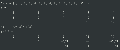
Figure 5. Row-Echelon Form of matrix A obtained using MATLAB

On the other hand, RREF is uniquely determined because it reduces the pivots and eliminates all the elements above the pivot.

In MATLAB, we can use the function rref() to obtain RREF.

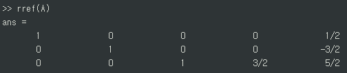
Figure 6. Reduced Row-Echelon Form of matrix A obtained using MATLAB

The usefulness of REF and RREF

RREF: Calculation of Inverse Matrix

When the vector $b$ in $Ax=b$ comes in various forms, you can solve the equations for all of them at once by performing Gaussian-Jordan elimination on an augmented matrix instead of solving them separately.

For example, let’s say you want to obtain solutions for the following three cases.

Then, instead of performing calculations three times for each case, you can construct an augmented matrix as follows and perform Gaussian-Jordan elimination to solve all three equations at once.

This is equivalent to solving the following matrix problem.

Now, what if we apply the fact that we can use an augmented matrix like this to the following matrix?

That is, the matrix $B$ should be multiplied behind the matrix $A$ to output the identity matrix as the result.

In other words, the matrix $B$ is the inverse matrix of $A$.

Therefore, applying Gauss-Jordan elimination to the augmented matrix above yields the reduced-row echelon matrix as follows:

Thus, we can calculate the inverse of $A$ as follows:

Solution Calculation through Row Operations

When solving a system of linear equations, we can obtain the solution by taking the constant multiple of an equation, adding or subtracting equations, or rearranging the order of equations.

And, as we saw in the Elementary Square Matrices, row operations are techniques that transfer the techniques applied to a system of linear equations to matrix operations. Row operations mean multiplying a row of a matrix by a constant, adding rows of a matrix together, and changing the order of rows.

When solving a system of linear equations, if we multiply an equation by a constant, add or subtract equations, or rearrange the order of equations, the solution remains the same. Therefore, even if we perform row operations, the solution remains the same.

So, suppose the original matrix is $A$, its REF is $U$, and its RREF is $R$. Then the solutions to $Ax=b$, $Ux=c$, and $Rx=d$ are all the same.

(Here, $c$ and $d$ are obtained by replacing $b$ in the right-hand side of the equation with $A$ transformed to $U$ or $R$.)

In other words, $A$, $U$, and $R$ are all row-equivalent.

In other words, we can say that the row space remains the same even if we perform row operations. However, the column space changes.

For example, suppose we want to solve the following system of equations:

This can be thought of as solving the following matrix equation:

However, even if we find the solution to $Ux=c$ after obtaining the REF, we can still find the same solution as the one for the above equation.

And if we obtain the RREF and find the solution to $Rx=d$, we can still find the same solution.

The equation that appears to be the easiest to solve for finding the solution is $Rx=d$, and we can easily see that

Discrimination of linear independence/dependence of row vectors

To determine whether two vectors $v_1$ and $v_2$ are linearly independent, you can perform the following process.

Consider the equation:

If this equation holds with non-zero values for $c_1$ and $c_2$, then the vectors $v_1$ and $v_2$ are linearly dependent. In other words, they are not linearly independent.

In other words, we can rearrange the equation as follows:

If there exist non-zero values for $c_1$ and $c_2$ that satisfy this equation, then $v_1$ and $v_2$ are scalar multiples of each other.

On the other hand, if the only values that satisfy $c_1 v_1 + c_2 v_2 = 0$ are $c_1 = 0$ and $c_2 = 0$, then $v_1$ and $v_2$ are linearly independent.

Finding the Row-Echelon Form or Reduced Row-Echelon Form of a matrix involves performing row operations.

If, during this process, a row becomes all zeros, then it means that this row is a linear combination of the other rows.

In other words, it means that this row is linearly dependent on the other rows.

For example, consider the matrix $A$ below:

If we perform the following row operation on the matrix:

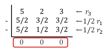
Figure 7. A row that is linearly dependent on other rows can be eliminated through row operations.

We can see that the third row can be reduced to all zeros. In other words, $r_3$ can be expressed as a linear combination of $r_1$ and $r_2$.