Prerequisites

To better understand this post, it is recommended that you have knowledge of the following:

• Sample and Sample Statistics
• Student’s t-test
• Null Hypothesis

Motivation

Sometimes we want to determine if there is a statistically significant difference between two groups. However, there are cases where it is difficult to use traditional parametric statistical methods. In such cases, we can consider the permutation test, one of the non-parametric tests.

The biggest advantage of parametric statistical methods is that they can solve problems using only parameters.

However, to do this, it is necessary to know the distribution of the population or statistics of the sample¹. If this condition is not satisfied, we cannot use parametric statistical methods.

In contrast, using the permutation test, one of the non-parametric tests, we can perform comparisons between sample groups even when the population distribution of the data does not follow a normal distribution or when unusual statistics are used.

In this post, let’s take a look at the background theory and practical usage of the permutation test.

Background Theory and Procedure of Permutation Test

Null Hypothesis of Permutation Test

Before we understand the background theory of the permutation test, let’s review what we mean when we say “there is a difference between two groups.”

When studying the null hypothesis and t-test, we often hear the phrase:

"Let's assume that two sample groups come from one population."

This is the “null hypothesis.” This time, we can observe the above statement slightly differently, and represent it as a picture, as follows.

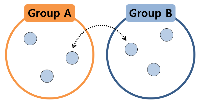
Figure 1. Two sample groups can be considered to be extracted from the same population

The above picture exaggerates the fact that all samples have the same value, but the essential point is as follows.

If two sample groups are extracted from the same population, even if the samples in the two groups are exchanged and statistically validated, there should be no difference between the two groups.

This part is the most essential null hypothesis of exchangeability that inspired the permutation test. Borrowing an expression from a textbook, it can be called null hypothesis of exchangeability.

That is, if the samples from the two groups really came from the same population, even if the samples are exchanged to calculate the statistics, there should be no difference between the two groups.

However, if two sample groups, as shown in the figure below, are extracted from completely different populations, it can be expected that the calculated value of the statistic will change significantly when the samples are exchanged.

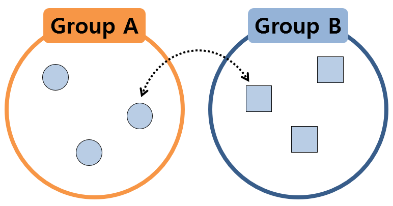
Figure 2. Two sample groups extracted from different populations

So, we will extract the statistics by shuffling the samples multiple times. And by checking the distribution of the values of the extracted statistics, we can estimate how large the value of the statistic calculated from the original given data is.

Procedure of Permutation Test

From now on, we will randomly shuffle the samples, rather than mixing them one pair at a time, and divide them into groups. In other words, it means that we will select the original data while considering the order.

This concept is called permutation, which is taught during high school probability class. Then, let’s calculate the statistic and draw a histogram.

Of course, if we just describe it in words like this, it is difficult to understand it immediately, so let’s take an example to understand it gradually.

Let’s assume that we have the sample data of two groups as follows:

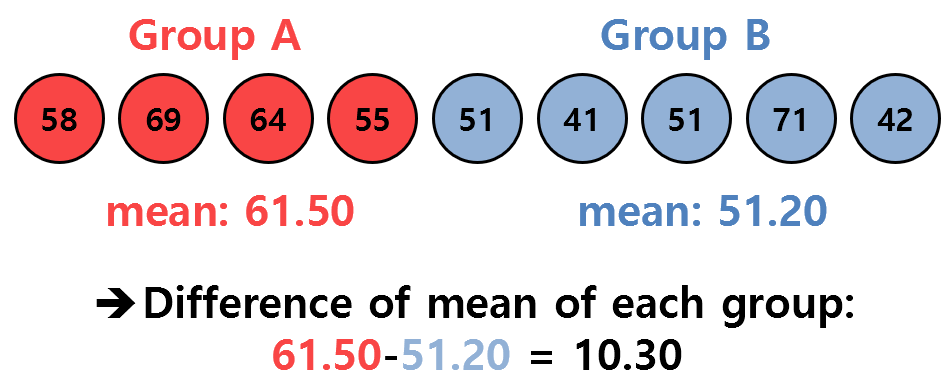
Figure 3. Sample data of two given groups and the statistic we want to observe (difference in mean)

What we want to know here is whether the difference in the means of the two groups, which is 10.30, is a value that can be statistically significantly large.

(That is, in this case, the difference in mean values of the two groups was used as the statistic. If necessary, any other statistic can be used…)

We cannot know from which population each group of samples came from, and since the sample size is too small, it is difficult to apply the central limit theorem, making it difficult to use the parametric test. Therefore, let’s use a permutation test according to the purpose of this post.

The ultimate goal is to create a distribution of the test statistic and see if the observed difference in the mean value, which is 10.30, is a significantly large value in the distribution.

To create the distribution, we select the original sample data given as follows:

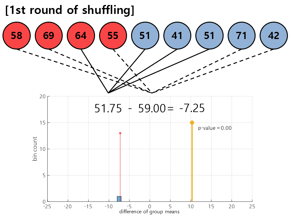
Figure 4. In the first round of shuffling, the data [3, 5, 6, 7], [1, 2, 4, 8, 9] were selected.

In permutation test, we shuffle the data several times and continuously draw the test statistic as a histogram. Figure 4 shows the shuffling result obtained in the first round.

As shown in the result, the data [3, 5, 6, 7] was assigned to the first group, and [1, 2, 4, 8, 9] was assigned to the second group, making it possible to calculate the difference in mean values between the newly assigned groups.

This mean value is plotted as a histogram, as shown in the bottom of Figure 4.

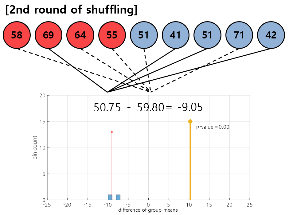
Figure 5. In the second round of shuffling, the data [2, 6, 7, 9], [1, 3, 4, 5, 8] were selected.

Figure 5 shows the result of the second round of shuffling. As in the first round, the samples are randomly assigned to each group, and the difference in mean values between the newly assigned groups is continuously added to the histogram.

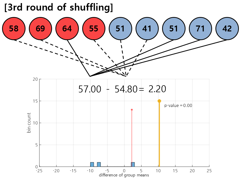
Figure 6. In the third round of shuffling, the data [3, 8, 7, 9], [1, 2, 4, 5, 6] were selected.

Figure 6 shows the result of the third round of shuffling. As in the first and second rounds, we calculate the difference in mean values between the randomly assigned samples in each group and plot them as a histogram.

By repeating the steps shown in Figures 4-6 multiple times, we can obtain a distribution as shown in the following video.

In the following video, the results of 100 shuffles are presented.

Figure 7. Permutation distribution obtained by performing shuffling up to 100 times.
This figure was created by modifying the figure in the Wikipedia entry for permutation test.

Finally, let’s calculate the p-value to see how high the value of 10.30 we were given ranks on the permutation distribution.

The p-value was calculated as the ratio of the number of values larger than 10.30 among the data obtained from shuffling to the total number of shuffles performed.

For example, suppose there were 13 shuffling results as follows:

[1, 2, 3, 4, 5, 6, 7, 8, 9, 10, 11, 12, 13]

Among them, the numbers larger than 10.30 are 11, 12, and 13, and the total number of shuffles is 13. Then,

\[3/13=0.2308\]

was assumed as the p-value.

What is the difference from Bootstrap?

In a previous blog post, there was a posting about Bootstrap.

Bootstrap is also a nonparametric statistical technique that allows us to examine the distribution of an estimator, similar to the permutation test.

The two main differences that can be identified are that Bootstrap is mainly used to determine the confidence interval of the estimator, while the permutation test was designed to test the null hypothesis. Additionally, while Bootstrap performs resampling with replacement, permutation test performs resampling without replacement.

References

• Mass univariate analysis of event-related brain potentials/field I: A critical tutorial review, David M. Groppe et al., Psychophysiology, 2011
• StackExchange: bootstrap vs permutation hypothesis test