※ This post is written using the results and source code of the GAN deep learning project in an art museum, available at http://www.yes24.com/Product/Goods/81538614 (in Korean).
※ The source code for this post can be found in Haesun Park’s GitHub repo.
In this post, we will discuss AutoEncoders (AE), which were one of the foundational concepts in deep learning theory, along with Restricted Boltzmann Machines (RBM).
RBM and AE have almost the same goal, which is to obtain latent factors related to data from the input layer (or visible layer) in the hidden layer.
This may sound a little complicated, but to put it simply, an AE is a neural network that compresses and then decompresses data.
So why compress and decompress data when you could just obtain the original data? Firstly, because we want the neural network to learn the compression method. In other words, we want to perform non-linear dimensionality reduction and represent the original high-dimensional data in a lower dimension.
There may be some loss of data in this process, but we can train a better AE by minimizing this loss through a process.
Secondly, an AE can be useful for generating previously unseen data.
As mentioned earlier, we can obtain a compressed lower-dimensional vector space. If we have a well-trained AE, we can select random points in this compressed space and then decompress them to generate previously unseen data.
This is because the AE has learned how to decompress the data represented in a lower dimension to a higher dimension.
These two tasks are called encoding and decoding, respectively. In other words, the compression process is called encoding, and the decompression process is called decoding. The parts that perform these tasks are called encoders and decoders, respectively.
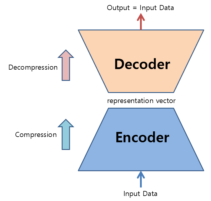
Figure 1. Structure and role of autoencoder
From a compression perspective: The role of an encoder
Compression of data can be viewed as similar to “dimensionality reduction”. However, the term “compression” is used instead of “dimensionality reduction” because the former involves non-linear dimensionality reduction, rather than linear projection or orthogonal projection used in linear dimensionality reduction.
Using an autoencoder (AE), we can compress data and obtain a representation vector as a result. One way to intuitively understand this representation vector is to draw it as a 2D or 3D vector.
In this blog post, we will apply an AE to the MNIST dataset to perform dimensionality reduction. The MNIST dataset contains hand-drawn images of digits from 0 to 9, with each image being 28x28 pixels in size.
The following image shows a visualization of the representation vectors obtained by compressing the 784-dimensional data (28x28) of the MNIST dataset into 2 dimensions, with different colors indicating different labels.
From the visualization, we can see that the data labeled as 0 (purple) are located in the upper-left corner and are separate from other label’s digits.
Furthermore, the data labeled with 1 are spread out in the lower-right corner and separated from the numbers labeled with other labels. On the other hand, the data that are not labeled with 0 or 1 are dispersed together in the center.
For now, let’s not worry too much about the fact that the representation vectors are not separated by each label, as we will discuss how to improve this result in the Variational AutoEncoder post.
Anyway, the role of the encoder in the AE is to compress high-dimensional data (in this case, 784-dimensional data) into a low-dimensional vector (here, 2-dimensional) that can represent the data.
By the way, let me mention one more new term: the vector space where the representation vector is displayed is called the latent space, which is a bit of a difficult term.
From the perspective of decompression: the role of the decoder
Now let’s think about AE from the perspective of the decoder.
The decoder takes an arbitrary representation vector in the latent space and “uncompresses” it to restore the original data in its original size.
In Figure 3 below, we can see the process of sampling an arbitrary representation vector from the 2-dimensional latent space in which the MNIST dataset is represented.
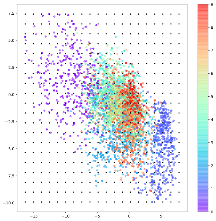
Figure 4. Sampling of arbitrary representation vectors in the 2-dimensional latent space of the MNIST dataset (black dots)
The “uncompressed” results of the sampled points are shown in Figure 5 below.
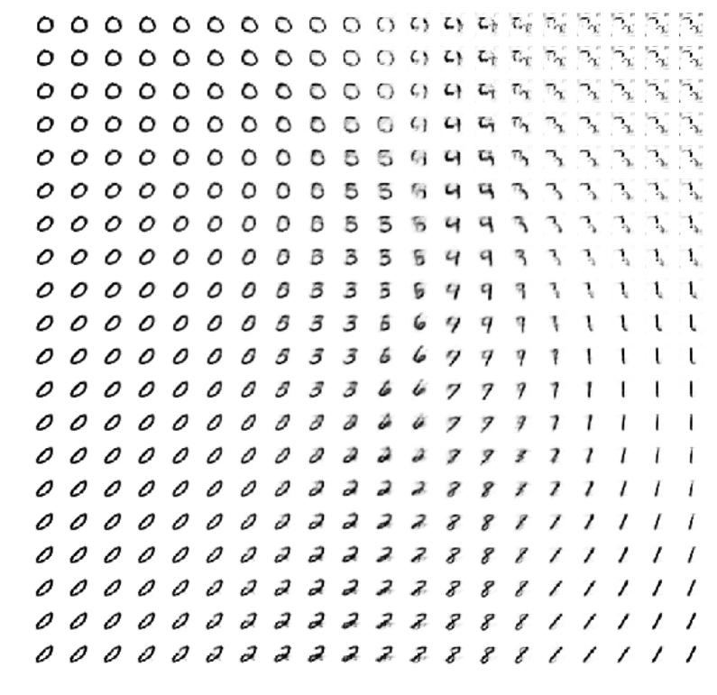
Figure 5. Results of decoding ("uncompressing") arbitrary representation vectors
As we can see in Figure 3, 0 and 1 are clearly separated and distinguished from other label numbers. This observation is consistent with the decoding result in Figure 4.
In other words, we can see that 0 and 1 are the most clearly distinguishable digits from other numbers.
On the other hand, we can observe new forms of data that do not look like digits, as well as some digits that are somewhat distinguishable in their form.
Another interesting point is that we can observe a smooth transition in the shape of the digits in the bottom row of Figure 4, as the digits transition from 0 to 2 to 8 to 1.
Output of AE
Could the AE perform the function of “providing the original input as output” faithfully?
Although it is not a completely satisfactory performance, it can be seen that it somewhat restores the original image.
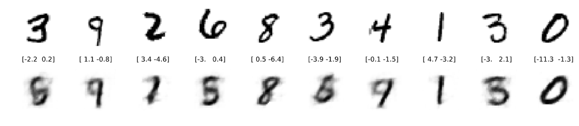
Figure 6. Example of a reconstructed image from input
Relationship between AE and Deep Learning?
The core content of deep learning is not just about “having deep neural network layers,” but rather about “what good effects occur when the layers become deeper.”
According to what is known, when the neural network is well trained, the layers closer to the input extract features of simple patterns, while as the layers become further away from the input (i.e., deeper), they learn and extract more abstract concepts and features.
At this point, the AE obtains a representation vector of the input dataset, and if we change our perspective, it is performing data abstraction. Since we are trying to squeeze the characteristics of the data into a small space, we need to create a latent space consisting of symbolic features.
Stacked AutoEncoder is the process of using AE to build deeper layers, and it is the idea that we can train a deep neural network by fine-tuning the abstract features of the input data obtained in this way.
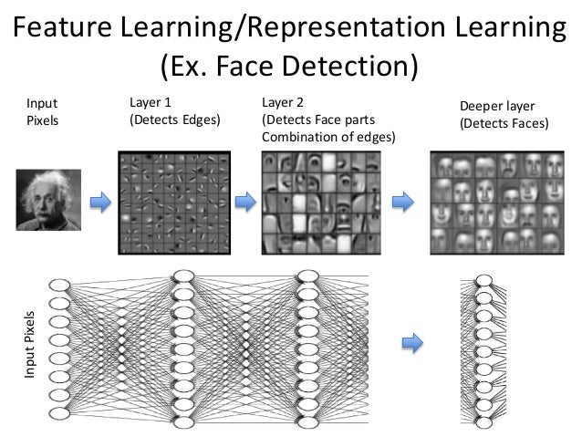
Figure 6. Deep neural networks learn to extract more abstract features in deeper layers.
Image source