In this article, we will learn about the normal vector of a parametric surface, which is essential to understanding the surface integral of a vector field.

To do this, we first need to understand the mathematical representation of a surface.

The equation of a curve represented by a single parameter

The parametric equation can generally be expressed as follows:

For a parameter $t$,

\[r(t) = \begin{bmatrix}x(t)\\y(t)\end{bmatrix}=x(t)\hat{i}+y(t)\hat{j}\]

Although we learn this concept in high school math, it can be difficult to understand the equation of a straight line (or curve) represented by a parameter at first glance.

The reason is that the functions we usually draw show both the input and output on the same plane (usually the input is represented on the $x$-axis, and the output is represented on the $y$-axis). This allows us to see how the output changes as the input changes at a glance.

However, the equation represented by a parameter only shows the output of the function. Therefore, it can be difficult to understand the output at a glance.

To understand the equation of a straight line (or curve) represented by a parameter more easily, we need to be able to show the changes in both the input and output simultaneously.

A parameter used to represent a straight line in real life is a scroll.

Figure 1. The scroll maps the current location on the screen to the desired location based on the position of the scroll.

As shown in Figure 1, when we move the scroll, the screen displaying the desired location mapped to the current position of the scroll is displayed.

That is, the scroll represents the domain of the parameter, and the location currently displayed on the screen represents the range.

Let’s represent a more complex function using this method, which simultaneously shows the domain of the parameter and the range of the function.

The applet below shows the function $r(t)$ represented using the parameter $t$.

\[r(t) = \begin{bmatrix} t\cdot \cos(2\pi t) \\ t\cdot \sin(2\pi t)\end{bmatrix}\]
Parametric equation of a curve with respect to t

In the applet above, we can see the changes from $t=0$ to $t=3$ represented on the slider, and how the results are mapped according to the changes of each $t$.

Tangent vectors of a curve expressed with a parameter

Moreover, curves expressed with parameters can also be differentiated like other functions.

The following graph shows the changes in the tangent vector as $t$ varies:

Tangent vector of a curve with respect to t

The tangent vector expressed with the parameter can be written as:

\[r'(t) = \begin{bmatrix} dx / dt \\ dy/dt\end{bmatrix}\]

This means that it shows how much $x(t)$ and $y(t)$ change when the parameter $t$ changes slightly.

Equation of a surface expressed with two parameters

So, how can we express the equation of a surface?

Generally, the equation of a surface requires two parameters.

The equation of a surface expressed with parameters can be written as:

\[r(u, v) = \begin{bmatrix}x(u,v) \\ y(u,v) \\ z(u,v) \end{bmatrix} = x(u,v)\hat{i} + y(u,v)\hat{j} + z(u,v)\hat{k}\]

As with understanding curves, if we set separate domains and ranges, we can express the surface as shown in the figure below.

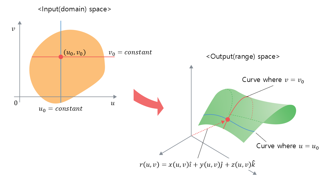
Figure 2. Input space and output space of a surface represented using parameterization

Firstly, since the equation of a surface is expressed using two parameters $u$ and $v$, the input space (domain) can be considered as a two-dimensional vector space.

In the output space (range), the value of the output function $r(u, v)$ is determined as $u$ and $v$ vary, and thus the position in a three-dimensional vector space is determined.

It is particularly noteworthy that if either $u$ or $v$ is fixed as a constant in the input space, a single curve is determined in the output space.

Tangent plane and normal vector of a surface represented using parameterization

If a surface can be determined using the equation with parameters, a small change $du$ or $dv$ in the $u$ or $v$ direction in the input space leads to a small change $dr$ in the output function $r$.

For example, if we consider the small change in $r$ caused by a small change in $u$ when $v$ is held constant, we can find the tangent vector of a curve on the surface as seen in Figure 1, and this process can be considered as the application of the concept of partial differentiation.

Therefore, we can express the ratio of these changes using the partial derivative symbol as follows:

\[\text{Rate of change of }r\text{ with respect to small changes in }u\Rightarrow \frac{\partial r}{\partial u} = r_u\] \[\text{Rate of change of }r\text{ with respect to small changes in }v\Rightarrow \frac{\partial r}{\partial v} = r_v\]

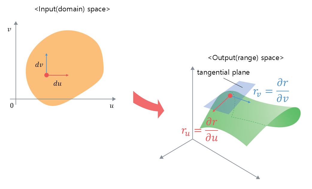
Figure 3. Rate of change in the output space with respect to small changes in the input space

If we can obtain two vectors in different directions at a point in the output space, we can determine a tangent plane, and the normal vector of the tangent plane can be expressed as the cross product of the two vectors.

Moreover, since the normal vector has only direction information without magnitude, we can calculate the normal vector of the surface as follows:

\[\hat{n} = \frac{r_u\times r_v}{|r_u\times r_v|}\]