Solutions to differential equations are often expressed in terms of exponential functions. Our question can be formulated as follows:
“Why are solutions to differential equations expressed using the Euler’s number e?”
This is because differential equations are a description of growth through feedback.
Prerequisites
To fully understand the content of this post, we recommend that you have a good understanding of the following:
Another Perspective on Differential Equations
So far, we have looked at differential equations from two perspectives: in Modeling Phenomena with Differential Equations, we saw differential equations as equations that involve derivatives, and in Direction Fields and Euler’s Method, we interpreted differential equations geometrically as a mapping of slopes for coordinates (x, y).
In this post, we want to look at differential equations from yet another perspective: continuous growth through feedback.
Feedback is the process of taking the output and using it as an input for the next iteration.

Figure 1. Block diagram of a system with input and feedback.
Differential equations describe growth over time. For example, consider the very simple differential equation below:
\[\frac{dx}{dt}=f(t, x)\]Let’s use the definition of the derivative to expand the derivative coefficient.
\[\lim_{h\rightarrow 0}\frac{x(t+h)-x(t)}{h}=f(t, x)\]The introduction of the concept of limit is the most difficult part in understanding the derivative coefficient.
We can replace the smallest value of $h$ with a small value such as $\Delta t$ that is easy to think about, and expand the equation further.
\[\Rightarrow \frac{x(t+\Delta t)-x(t)}{\Delta t} = f(t, x)\]Then we see the following equation:
\[x(t+\Delta t) = x(t) + \Delta t f(t, x) % Equation (4)\]This equation means that when we increase the current value $x(t)$ by $\Delta t f(t, x)$, we get the next step’s value $x(t+\Delta t)$.
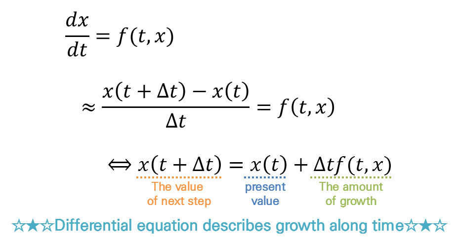
Figure 2. Differential equations describe how the function's value changes at each step through continuous growth.
The time step $\Delta t$ we consider here is related to continuous growth, as when we consider a very small time unit for a real differential equation.
Continuous growth through accumulation
Let’s look at Equation (1) again.
Looking at Equation (1, the left-hand side is a formula for the growth rate of $x(t)$ every time, and the right-hand side tells us how that growth rate is calculated.
The solution to a differential equation is the result obtained by accumulating (i.e., integrating) the given amount of growth from the initial value.
It is very important that the dependent variable $x$ is included on the right side of Equation (1), as it is only then that we can call it ‘continuous growth through accumulation’.
If only an equation for the independent variable $t$ is included on the right side, it is difficult to regard this differential equation as a description of continuous growth through accumulation.
To understand this, let’s think about the difference between the two equations below.
\[\frac{dx}{dt}=f(t) % 식 (5)\] \[\frac{dx}{dt}=f(x) % 식 (6)\]Equations (5) and (6) are both recipes for growth. This is because the left-hand side represents the growth rate, and the right-hand side describes the polynomial that represents that growth rate.
In other words, it describes how much growth should occur at each point in time.
However, if we expand equations (5) and (6) like equation (4), we get the following:
\[Equation(5)\Rightarrow x(t+\Delta t)=x(t)+\Delta t f(t)\] \[Equation(6)\Rightarrow x(t+\Delta t)=x(t)+\Delta t f(x)\]Equation (5) is a recipe where the change in growth rate over time is applied when transitioning from the current value to the next value, while Equation (6) is a recipe where the growth rate related to the current value is applied.
In other words, to have growth through accumulation, there must be a function related to x on the right-hand side of equation (1).
Continuous growth through accumulation using Euler’s number
So, how does the expression of continuous growth through accumulation using Euler’s number relate to the fact that the solution to differential equations is often expressed using the function $e^t$?
In the Euler’s number post, it was mentioned that the natural constant $e$ is the growth rate itself when it comes to continuous growth.
What example did we examine to understand continuous growth?
We thought about “continuous growth through accumulation,” where we obtain the next growth value by multiplying the growth rate by the accumulated output at each point in time, just like when applying the concept of compound interest.
Let’s consider the following picture as a specific example:
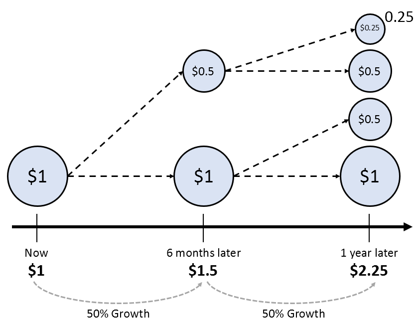
Figure 2. An example of discontinuous growth that was examined during the understanding of Euler's number
In the above picture, we applied discontinuous growth twice. We obtained the result by multiplying the number 1 by 1.5 and then multiplying it by 1.5 again.
We also apply a similar method when solving differential equations.
In fact, by solving the differential equation that includes a function of x on the right side of equation (1), we can see that the solution is expressed as Euler’s number, e.
For a simple example, for the following differential equation:
\[\frac{dx}{dt}=x\]If we make the left side all in terms of x and the right side all in terms of t, then we can see that it is:
\[\frac{1}{x}dx = dt\]And if we integrate both sides:
\[\int \frac{1}{x}dx=\int dt\]Here, the indefinite integral of 1/x is natural logarithm:
\[\Rightarrow \ln(x)=t+C\]Here, C is the constant of integration.
Therefore:
\[x(t)=Ce^t\]The Meaning of Homogeneous Differential Equations
As we study differential equations, we come across the terms homogeneous differential equations and nonhomogeneous differential equations.
A homogeneous differential equation corresponds to equation (6) in our example. Rewriting equation (6) to put all x terms on the left side and all t terms on the right side gives us the following:
\[\frac{dx}{dt}-f(x) = 0 % Equation (14)\]If we examine this equation closely, we can see that there are no terms in t on the right side.
On the other hand, a nonhomogeneous differential equation corresponds to equation (5) in our example. Rewriting equation (5), we get:
\[\frac{dx}{dt}=f(t) % Equation (15)\]In this equation, there is still a term in t on the right side.
What does this mean?
If we compare equation (15) with equation (14), the difference is that equation (15) means that the law of how $x(t)$ changes over time depends not only on the current value of the function, but also on an additional parameter $t$.
In other words, the equation in (14) sets up an autonomous system with no external input. On the other hand, equation (15) represents a system that receives external input and the system’s rules are changing constantly.
Here, the meaning of homogeneous differential equations seems to come from the translation of the word “homogeneous”, which means “the same” or “equal” in Korean.
According to dictionary.com, in the mathematical sense, “homogeneous” means “having a common property throughout”.
Therefore, we can understand that homogeneous differential equations refer to systems that maintain a “constant” or “consistent” system that does not change over time, even as time goes by.
In other words, the essential meaning of a homogeneous differential equation is that it establishes its own system without external input.